Forecasting Ability But No Profitability:
An Empirical Evaluation of Genetic
Algorithm-optimised Technical Trading
Rules
Pereira, Robert
1999
Online at
https://mpra.ub.uni-muenchen.de/9055/
An Empirical Evaluation of Genetic
Algorithm-optimised Technical Trading Rules
Robert Pereira
School of Business LaTrobe University
Bundoora, Victoria, Australia 3083 [email protected]
Abstract. This paper evaluates the performance of several popular technical
trad-ing rules applied to the Australian share market. The optimal tradtrad-ing rule parame-ter values over the in-sample period of 4/1/82 to 31/12/89 are found using a genetic algorithm. These optimal rules are then evaluated in terms of their forecasting abil-ity and economic profitabilabil-ity during the out-of-sample period from 2/1/90 to the 31/12/97. The results indicate that the optimal rules outperform the benchmark given by a risk-adjusted buy and hold strategy. The rules display some evidence of forecasting ability and profitability over the entire test period. But an examination of the results for the sub-periods indicates that the excess returns decline over time and are negative during the last couple of years. Also, once an adjustment for non– synchronous trading bias is made, the rules display very little, if any, evidence of profitability.
1
Introduction
Forecasting the future direction of share market prices is an important, but difficult exercise. Both technical and fundamental analysis have been used for this purpose, with varying success. Initial studies of technical analysis by [2] and [16] were unable to find evidence of profitability and thus concluded that technical analysis is not useful. More recently, there has been a renewed interest in this topic; see [7,10,3].
Under an efficient market it is expected that prices follow a random walk and thus past prices cannot be used successfully to forecast future prices. There-fore, the most appropriate investment strategy is the buy and hold strategy which consists of holding the market portfolio. It is not expected that any other strategy can consistently beat or outperform the market.
Although criticized by economists, most notably [25], technical analy-sis has received an increasing amount of attention by academics. Numerous studies examining technical trading rules applied to various shares and share market indices, have uncovered evidence of predictive ability and profitability; see [28,8,6,19,27]. There are also studies which have found some evidence of predictive ability but no profitability once reasonable adjustments are made for risk and trading costs; see [12,20,7,10,3].
The majority of these studies have examined trading rules where both the rules and their parameter values were chosen arbitrarily. However this approach leaves these studies open to the criticisms of data-snooping and the possibility of a survivorship bias; see [23] and [9] respectively. By choosing trading rules based on an optimisation procedure utilising in-sample data and testing the performance of these rules out-of-sample, this bias can be avoided or at least reduced. This approach is taken by [26] and [3], by employing a genetic programming approach to discover optimal technical trading rules for the foreign exchange market and US share market respectively.
In this paper the forecasting ability and economic profitability of some popular technical trading rules applied to the Australian share market are in-vestigated using a standard genetic algorithm optimisation procedure.1 The
approach adopted in this study differs from the genetic programming ap-proach for two reasons. First, since the objective of this study is not to discover new trading rules but rather to examine popular, commonly used trading rules.2 Second, there is a potential problem associated with the use
of genetic programming, since this artificial intelligence technique was only recently developed by [21]. Therefore it is unrealistic to evaluate the perfor-mance of trading rules discovered by the genetic programming approach prior to the date of the development of this technique.
The next section of the paper describes the technical trading rules ex-amined in this study. Section 3 develops the genetic algorithm methodology used in trading rule optimisation. Section 4 explains the performance mea-sures that are used to evaluate trading rule forecasting ability and economic profitability. Section 5 considers an empirical investigation of the performance
1
To the author’s knowledge there is only one other study considering the perfor-mance of technical trading rules applied to the Australian share market. The performance of the filter rule applied to various individual Australian shares was examined by [4], who was unable to find any significant evidence of profitability.
2
of the genetic algorithm-optimised technical trading rules applied to the Aus-tralian share market. Finally, Section 6 provides some conclusions and direc-tions for possible future research.
2
Technical Trading Rules
Trading rules are used by financial market traders to assist them in deter-mining their investment or speculative decisions. These rules can be based on either technical or fundamental analysis. This study considers only rules based on technical indicators. A technical indicator is a mathematical for-mula that transforms historical data on price and/or volume into a single number. These indicators can be combined with price, volume or each other to form trading rules. Some of the more popular technical indicators used by traders include: channels, filters, momentum, moving averages and rela-tive strength indices. Reference [1] provides an excellent description of the different technical indicators used in trading.
2.1 Determination of the investment position
Trading rules return either a buy or sell signal which together with a particu-lar trading strategy determines the trading position that should be taken in a security or market. The trading strategy considered in this study is based on a simple market timing strategy, consisting of investing total funds in either the share market or a risk free security. If share market prices are expected to increase on the basis of a buy signal from a technical trading rule, then the risk free security is sold and shares are bought. However, if the rule returns a sell signal, it is expected that share market prices will fall in the near future. As a result, shares are sold and the proceeds from the sale invested in the risk free security.3
2.2 Different types of rules
Two general types of technical trading rules are considered - rules based on either moving averages or order statistics.
Moving average rules Moving averages are used to identify trends in prices. A moving average (M A) is simply an average of current and past prices over a specified period of time. An M Aof lengthθis calculated as
3
M At(θ) =1
θ
θ−1
i=0
Pt−i (1)
where
∀θ∈ {1,2,3, ...}.
By smoothing out the short-term fluctuations or noise in the price series, the
M Ais able to capture the underlying trend in the price series over a particular period of time. An M A can be used to formulate a simple trend-following rule also referred to as a momentum strategy.
A simpleM Arule can be constructed by comparing price to its trend, as represented by theM A. If the price rises above theM A, then the security is bought and held until the price falls below theM Aat which time the security is sold. This simple rule can be modified to create the filteredM Arule and the doubleM Arule. A filteredM Arule is similar to the simpleM Arule, except it includes a filter which accounts for the percentage increase or decrease of the price relative to itsM A. The purpose of this filter is an attempt to reduce the number of false buy and sell signals, which are issued by a simple M A
rule when price movement is nondirectional. This rule operates by returning a buy signal if the price rises byX percent above theM Aand then returning a sell signal only when the price falls by X percent below the M A at which time the security is sold. In contrast to the previous two rules, a doubleM A
rule compares two M As of different lengths. With this rule if the shorter lengthM A rises above the longer length M A from below then the security is bought and held until the shorterM Afalls below the longerM Aat which time the security is sold.
A more general M A rule can be specified by considering two moving averages and a filter.4 This Generalised MA (GMA) rule can be represented
by the binary indicator function
S(Θ)t=M At(θ1)−
1 + (1−2St−1)
θ3
104
M At(θ2)
>0, 1
≤0, 0 (2)
where
∀θ1, θ2∈ {1,2,3,4, ...}, θ1< θ2 ∀θ3∈ {0,1,2, ...}
and theM Aindicator is defined by Equation 1. This function returns either a one or zero, corresponding to a buy or sell signal respectively, which indicates
4
the trading position that should be taken at timet. The lengths of the short and longM As are given by parametersθ1andθ2,which represent the number
of days used to calculate the M As. The parameter θ3 represents the filter
parameter in terms of basis points; where one hundred basis points equivalent to one percent.
The three differentM Arules discussed above are nested within the GMA rule. These rules can be derived individually by imposing certain restrictions on Equation 2:
1.Simple MA: θ1= 1,θ2>1 andθ3= 0
S(Θ)t=Pt−M At(θ2)
>0, 1
≤0, 0
2.Filtered MA:θ1 = 1,θ2>1 andθ3 >0
S(Θ)t=Pt−
1 + (1−2St−1)
θ3
104
M At(θ2)
>0, 1
≤0, 0
3.Double MA: 1< θ1< θ2andθ3 = 0
S(Θ)t=M At(θ1)−M At(θ2)
>0, 1
≤0, 0.
Rules based on order statistics Technical trading rules can also be based on order statistics, such as the maximum and minimum prices over a specified period of time. The filter and channel rules are two examples which use local maximum and minimum prices. Reference [8] refer to this rule as the trading range break-out rule. The maximum price Pmax
t (φ) and the minimum price
Pmin
t (φ) at timet given a historical price series consisting ofφobservations are
Ptmax(φ) =M ax[Pt−1, ..., Pt−φ] (3)
Ptmin(φ) =M in[Pt−1, ..., Pt−φ] (4)
where
∀φ∈ {1,2,3, ...}.
defined using the maximum (or minimum) price over the most recent histor-ical period of prices consisting of φ observations as defined by Equations 3 and 4 respectively. This rule returns a buy (or sell) signal when price breaks through its current resistance (or support) level from below (or above) to above (or below) this level.
The filter rule is based on the idea that when price rises above (or drops below) a certain level, it will continue to rise (or fall) for some period of time. The filter rule operates by returning a buy signal when price increases by X percent above a previous low and a sell signal once the price falls by X percent below a previous high. The original filter rule of Alexander (1964) defines the previous low (or high) implicitly using the minimum (or maximum) price from a historical series commencing on the date of the most recent transaction.
The filter rule can be generalised by explicitly choosing the amount of data to use in order to determine the previous low or high. This can be done by introducing a parameterφwhich specifies a fixed length for the historical price series used to calculate the maximum or minimum price, similar to the channel rule. Furthermore the original channel rule as outlined above, can also be generalised by introducing a filter parameter. Similar to the filtered
M A rule, this rule will only return a buy (or sell) signal if the price exceeds the maximum (or minimum) price byX percent.
Since both the channel and filter rules use order statistics, these two rules can be nested within a single decision rule. This Generalised Order Statistic (GOS) rule is represented by the indicator function
S(Φ)t=Pt−
1 + (1−2St−1)
φ2
10−4
(Ptmax(φ1))
a
Ptmin(φ1)
b>0, 1
≤0, 0 (5)
where
a=φ3St−1+ (1−φ3)(1−St−1)
b=φ3(1−St−1) + (1−φ3)St−1
∀φ1, φ2∈ {1,2,3, ...}.
The parameterφ1represents the length of the historical price series used in
determining either the maximum or minimum price,φ2is the filter parameter
given in basis points andφ3 is a binary parameter defined as
φ3=
1, Filter rule
where the value one and zero represent the filter and channel rules respec-tively. The rule can be generalised further by allowing the parameterφ1 to
be derived either implicitly (as is the case with the channel rule) or explicitly (as is the case with the filter rule).
The filter and channel rules outlined above, can be derived from the GOS rule by imposing certain restrictions on Equation 5:
1. Filter rule; φ1 = number of days since last transaction, φ2 >0 and
φ3= 1
St=Pt−
1 + (1−2St−1)
φ2
10−4
(Ptmax(φ1))St−1Pmin t (φ1)
(1−St−1)
>0, 1
≤0, 0
2.Channel rule;φ1>0,φ2= 0 andφ3= 0
St=Pt−(Ptmax(φ1))(1−St−1)Pmin t (φ1)
St−1
>0, 1
≤0, 0
3
Genetic Algorithm Methodology
3.1 Optimisation
The choice of technical trading rule parameter values has a profound impact on the profitability of these rules. In order to maximise trading rule prof-itability, parameter values must be chosen optimally. In this optimisation problem, it is important to be aware of two issues. First, there are a large number of possible parameter values. Second, the profit surface is charac-terised by multiple optima; see [26] and [3]. Genetic algorithms are a very efficient and effective approach to this type of problem.
Efficiency refers to the computational speed of the optimisation technique. Through a recombination procedure known as crossover and by maintaining a population of candidate solutions, the genetic algorithm is able to search quickly through the profitable areas of the solution space. Effectiveness refers to the global optimisation properties of the algorithm. Unlike other search or optimisation techniques based on gradient measures, a genetic algorithm avoids the possibility of being anchored at local optima due to its ability to introduce random shocks into the search process through mutations. Since a genetic algorithm is an appropriate global optimisation method, it can be used to search for the optimal parameter values for the GMA and GOS trading rules given by Equations 2 and 5 respectively.5
Genetic algorithms were originally developed by [18]. They are a class of adaptive search and optimisation techniques based on an evolutionary
5
process. By representing potential or candidate solutions to a problem using vectors consisting of binary digits or bits, mathematical operations known as crossover and mutation, can be performed. These operations are analogous to the genetic recombinations of the chromosomes in living organisms. By performing these operations, generations of new candidates can be created and evolved over time through an iterative procedure. However, there do exist restrictions on the process of crossover so as to ensure that better performing candidates are evolved over time. Similar to the theory of natural selection or survival of the fittest, the better performing candidates have a better than average probability of surviving and reproducing relative to the lower performing candidates which eventually get eliminated from the population. The performance of each candidate can be assessed using a suitable objective function. A selection process based on performance is applied to determine which of the candidates should participate in crossover, and thereby pass on their favourable traits to future generations. It is through this process of “survival of the fittest” that better solutions are developed over time. This evolutionary process continues until the best (or better) performing individual(s), consisting of hopefully the optimal or near optimal solutions, dominate the population.6
3.2 Problem representation
Potential solutions to the problem of optimisation of the parameters of the GMA rule defined in Equation 2 can be represented by the vector
y1= [θ1, θ2, θ3]. (7)
For the GOS rule given by Equation 5, candidates can be represented by the vector
y2= [φ1,φ2, φ3,φ4] (8)
whereφ3is defined above given by Equation 6, whileφ4is a dummy variable
defined by
φ4=
1,φ1 is determined implicitly
0,φ1 is determined explicitly. (9)
In order to use a genetic algorithm to search for the optimal parameter values for the rules considered above, potential solutions to this optimisation
6
problem are represented using vectors of binary digits. Binary representa-tion is necessary in the standard genetic algorithm for the applicarepresenta-tion of the recombination operations. These vectors also known as strings, are linear combinations of zeros and ones, for example [0 1 0 0 1]. A binary representa-tionx= [x1, x2, x3, ..., xn] is based on the binary number system which has a
corresponding equivalent decimal value given byn
i=1(2n−i)xi. For example, the decimal equivalent of the vector [0 1 0 0 1] = (24×0) + (23 ×1) + (22 ×0) + (21 ×0) + (20 ×1) = 8 + 1 = 9.
Binary representation of the GMA rule The periodicity of the two
M As have a range defined by 1 < θ1 ≤ L1 and 2 < θ2 ≤ L1, where L1
represents the maximum length of the moving average. The filter parameter has a range given by 0≤θ3 ≤L2, whereL2 represents the maximum filter
value. For this studyL1= 250 days andL2= 100 basis points.7
In order to satisfy the limiting values given above, the binary representa-tions forθ1andθ2are each given by a vector consisting of eight elements. For
the filter parameter (θ3) a seven bit vector is required. Therefore, the binary
representation for the GMA rule can be defined by a row vector consisting of twenty three elements stated as
x1= [x11,x12,x13] (10)
where
x11= subvector consisting of eight elements (binary representation ofθ1)
x12= subvector consisting of eight elements (binary representation ofθ2)
x13= subvector consisting of seven elements (binary representation ofθ3).
Binary representation of the GOS rule The parameter on the chan-nel rule φ1 represents the number of the most recent historical observations
used to calculate either the maximum or minimum price. This parameter is restricted to the values 1≤φ1 ≤250. Therefore, the binary representation
is given by a vector consisting of eight elements. The range for φ2 is given
by 0 < φ2 ≤1000 basis points. Thus a vector consisting of ten elements is
used and the decimal equivalent values are restricted to the desired range. Therefore, the binary representations for the order statistics based rule can be defined by a row vector consisting of twenty elements stated as
x2= [x21,x22,x23,x24] (11)
7
where
x21= subvector consisting of eight elements (binary representation ofφ1)
x22= subvector consisting of ten elements (binary representation ofφ2)
x23= subvector consisting of one element (binary representation ofφ3)
x24= subvector consisting of one element (binary representation ofφ4).
3.3 Objective function
The ultimate goal of the genetic algorithm is to find the combination of bi-nary digits for the two vectorsx1 andx2, representing the parameter values
given byy1andy2, which maximises an appropriate objective function. Each
candidate’s performance can be assessed in terms of this objective function, which can take numerous forms depending upon specific investor preferences. Given that individuals are generally risk averse, performance should be de-fined in terms of both risk and return. The Sharpe ratio is an example of a measure of risk-adjusted returns. The Sharpe ratio is given by
SR= r
σ√Y (12)
where r is the average annualised trading rule return, σ is the standard deviation of daily trading rule returns, while Y is equal to the number of trading days per year. This formulation is actually a modified version of the original Sharpe ratio which uses average excess returns, defined as the difference between average market return and the risk-free rate.
Trading rules as defined by the indicator functions given in Equations 2 and 5, return either a buy or sell signal. These signals can be used to divide the total number of trading days (N), into days either “in” the market (earning the market rate of return rmt) or “out” of the market (earning the risk-free rate of returnrf t). Thus the trading rule return over the entire period of 0 to N can be calculated as
rtr= N
t=1
St−1rm,t+ N
t=1
(1−St−1)rf,t−T(tc) (13)
where
rm,t= ln
P
t
Pt−1
market. An adjustment for transaction costs is given by the last term on the right hand side of Equation 13 which consists of the product of the cost per transaction (tc) and the number of transactions (T). Transaction costs of 0.2 percent per trade are considered for the in-sample optimisation of the trading rules.
3.4 Operations
Selection, crossover and mutation are the three important mathematical oper-ations in any genetic algorithm. It is through these operoper-ations that an initial population of randomly generated solutions to a problem can be evolved, through successive generations, into a final population consisting of a poten-tially optimal solution. The search process which ensues is highly efficient and effective because of these operations.
Selection involves the determination of the candidates for participation in crossover. The genitor selection method, a ranking-based procedure devel-oped by [30], is used in the genetic algorithm employed in this study. This approach involves ranking all candidates according to performance and then replacing the worst performing candidates by copies of the better performing candidates. In the genetic algorithm developed in this paper a copy of the best candidate replaces the worst candidate.
The method by which promising (better performing) candidates are com-bined, is through a process of binary recombination known as crossover. This ensures that the search process is not random but consciously directed into promising regions of the solution space. As with selection there are a num-ber of variations, however single point crossover is the most commonly used version and the one adopted in this study.
To illustrate the process of crossover, assume that two vectorsA= [1 0 1 0 0] andB= [0 1 0 1 0] are chosen at random and that the position of parti-tioning is randomly chosen to be between the second and third elements of each vector. Vectors A and B can be represented as 1 0... 1 0 0
= [A1 A2]
and 0 1... 0 1 0
= [B1 B2] respectively, in terms of their subvectors.
Recom-bination occurs by switching subvector A2 with B2 and then unpartioning
both vectors A and B, producing two new candidates C = [1 0 0 1 0] and
D= [0 1 1 0 0].
probability of this occurrence is normally very low, so as to not unnecessarily disrupt the search process.
This operation can be illustrated by an example. Assume that the third element in vectorC = [1 0 0 1 0] undergoes mutation. The outcome of this operation changes the binary representation of vectorC slightly, producing a new candidate represented by E= [1 0 1 1 0].
3.5 Procedure
The genetic algorithm procedure can be summarised by the following steps:
1. Create an initial population of candidates randomly. 2. Evaluate the performance of each candidate.
3. Select the candidates for recombination. 4. Perform crossover and mutation.
5. Evaluate the performance of the new candidates.
6. Return to step 3, unless a termination criterion is satisfied.
The last step in the genetic algorithm involves checking a well-defined termination criterion. If this criterion is not satisfied, the genetic algorithm returns to the selection, crossover and mutation operations to develop further generations until this criterion is met, at which time the process of the cre-ation of new genercre-ations is terminated. The termincre-ation criterion adopted, is satisfied when either one of the following conditions is met:
1. the population converges to a unique individual,
2. a predetermined maximum number of generations is reached,
3. there has been no improvement in the population for a certain number of generations.
This latter condition ensures that the genetic algorithm cannot continue in-definitely.
3.6 Parameter settings
The genetic algorithm has six parameters settings {b, p, c, m, Gmax1 , Gmax2 },
defined as:
b= number of elements in each vector,
p= number of vectors or candidates in the population,
c= probability associated with the occurrence of crossover,
m= probability associated with the occurrence of mutation,
Gmax
1 = maximum number of generations allowed,
Gmax
2 = maximum number of iterations without improvement.
Table 1.Genetic Algorithm Parameters
Rule b p c m Gmax 1 G
max 2
GMA 23 150 0.6 0.005 250 150 GOS 20 150 0.6 0.005 250 150
explanation of these results. The greater the rate of convergence the lower the computational time that is required to reach the solution. However, if the rate of convergence is too rapid the solution space is not adequately searched, potentially missing the optimal solution (or better solutions to the one found).
Table 1 displays the parameter values that are used by the genetic al-gorithm for each of the trading rules. The choice of b values was discussed above in Section 3.1, while the choice of values forp,c,m, Gmax1 andGmax2
was guided by previous studies (see [5], Chapter 7) and experimentation with different values.
4
Performance evaluation
4.1 Economic profitability
The true profitability of technical trading rules is hard to measure given the difficulties in properly accounting for the risks and costs associated with trading. Trading costs include not only transaction costs and taxes, but also hidden costs involved in the collection and analysis of information. Trans-action costs of 0.1 percent per trade are used to investigate trading rule performance. Since according to [28], large institutional investors are able to achieve one-way transaction costs in the range of 0.1 to 0.2 percent. However, given that different individuals face different levels of transaction costs, the break-even transaction cost is also reported in the results section; see [6]. This is the level of transaction costs which offsets trading rule revenue with costs, leading to zero trading profits.
rbh= N
α
t=1
rf,t+ (1−α) N
t=1
rm,t−2(tc) (14)
whereαis the proportion of trading days that the rule is out of the market. This return represents the expected return from investing in both the risk-free asset and the market according to the weightsαand (1−α) respectively. There is also an adjustment for transaction costs incurred due to purchasing the market portfolio on the first trading day and selling it on the last day of trading.
Therefore, trading rule performance relative to the benchmark can be measured by excess returns
XR=r−rbh (15)
where r represents the total return for a particular trading rule calculated from Equation 13 and rbh is the return from the appropriate benchmark strategy given by Equation 14Since investors and traders also care about the risk incurred in deriving these returns, a Sharpe ratio based on excess returns can be calculated using Equation 12, wherer represents annualised excess returns given by Equation 15 and σ is the standard deviation of the daily excess returns.
4.2 Predictive ability
To investigate the statistical significance of the forecasting power of the buy and sell signals, traditional t tests can be employed to examine whether the trading rules issue buy (or sell) signals on days when the return on the market is on average higher (or lower) than the unconditional mean return for the market.
The t-statistic used to test the predictive ability of the buy signals is
tbuy=
rbuy− rm
σN1
buy + 1
N
(16)
whererbuyrepresents the average daily return following a buy signal andNbuy
is the number of days that the trading rule returns a buy signal. The null and alternative hypotheses can be stated as
H0: rbuy≤ rm
Similarly, a t-statistic can be developed to test the predictive ability of the sell signals. To test whether the difference between the mean return on the market following a buy signal and the mean return on the market following a sell signal is statistically significant, a t-test can be specified as
tbuy−sell=
rbuy− rsell
σN1
buy + 1
Nsell
(17)
where the null and alternative hypotheses are
H0: rbuy− rsell≤0
H1: rbuy− rsell>0.
Another test of whether the rules have market timing or forecasting ability is based on an approach suggested by [13]. This test is based on the following regression
rm,t−rf,t=α+βSt+εt (18)
where rm,t and rf,t are the return at time t for the risky asset or market portfolio and the risk-free security respectively, εt is a standard error term andStis the trading rule signal. To test whether a particular rule has market timing ability the regression given in Equation 18 is estimated using OLS and the following hypothesis test is conducted
H0:β= 0, no market timing ability
H1:β >0, positive market timing ability.
4.3 Statistical Significance
The bootstrap method proposed by [15] has been applied in finance for a wide variety of purposes; see [24]. Reference [22] use this method for the purpose of testing the significance of trading rule profitability, while [8] use trading rules on bootstrapped data as a test for model specification. In this study, a bootstrap approach similar to [22] is used to test the significance of both the predictive ability and the profitability of technical trading rules.
To use the bootstrap method a data generating process (DGP) for market prices or returns must be specified a priori. The DGP assumed for prices in this study is the simple random walk with drift
lnPt+1=µ+ lnPt+εt (19)
where µ represents the drift in the series, lnP is the natural logarithm of the price andε is the stochastic component of the DGP. Since continuously compounded returns are defined as the log first difference of prices, then the above DGP given in Equation 19 implies an IID normal process with a mean of zero for returns.
The bootstrap method can be used to generate many different return series by sampling with replacement from the original return series. The bootstrap samples created are pseudo return series that retain all the dis-tributional properties of the original series, but are purged of any serial de-pendence. Each bootstrap sample also has the property that the DGP of prices is a random walk with drift. From each bootstrap a corresponding price series can be extracted, which can then be used to test the significance of the predictive ability or profitability of a particular rule. This is done by applying the rule to each of the pseudo price series and calculating the empir-ical distribution of the trading rule profits or the statistic of interest. P-values can then be calculated from this distribution.
To test the significance of the trading rule excess returns the following hypothesis can be stated
H0: XR ≤ XR ∗
H1: XR > XR∗.
Under the null hypothesis, the trading rule excess return (XR) calculated from the original series is less than or equal to the average trading rule return for the pseudo data samples (XR∗). The p-values from the bootstrap
procedure are then used to determine whether the trading rule excess returns are significantly greater than the average trading rule return given that the true DGP is a random walk with drift. In a similar way, the market returns following buy and sell signals and the Sharpe ratio can also be bootstrapped to test the significance of the predictive ability and profitability of the trading rule studied.
The bootstrap procedure involves the following steps:
1. Create Z bootstrap samples, each consisting ofN observations, by sam-pling with replacement from the original return series.
2. Calculate the corresponding price series for each bootstrap sample given that the price next period isPt+1 =exp(rt+1)Pt.
3. Apply the trading rule to each of theZ pseudo price series.
4. Calculate the performance statistic of interest for each of the pseudo price series.
5
An empirical application
5.1 Data
The data consists of the daily closing All Ordinaries Accumulation index and the daily 90 day Reserve Bank of Australia bill dealer rate. The data is collected over the period 4/1/1982 to 31/12/97, consisting of 4065 obser-vations.8 For the purpose of avoiding the possibility of data-snooping, the
total period is split into an in-sample optimisation period from 4/1/1982 to 31/12/89 and an out-of-sample test period from 2/1/1990 to 31/12/97.
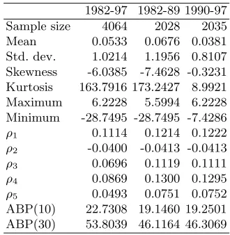
Table 2 provides summary statistics for the continuously compounded daily returns (rm) on the All Ordinaries index.9 The return series has
char-acteristics common to most financial time series and the results are broadly consistent with previous studies. The autocorrelation coefficients are also reported for the first five lags. These coefficients show evidence of highly significant low-order positive autocorrelation.10 Significant first-order serial
correlation in share indices is a well known stylized fact due to the inclusion of thinly-traded small shares in share market indices. Therefore, this result is not surprising given that the All Ordinaries Accumulation index is comprised of over 300 shares, which includes a significant amount of small shares. There also appears to be significant higher order serial correlation as indicated by the heteroscedasticity-adjusted Box-Pierce Q statistic (ABP). These results seem to be consistent across the in-sample optimisation and out-of-sample test periods.
5.2 Trading rule parameter values
A genetic algorithm was programmed and then used to search for the optimal parameter values using the All Ordinaries Accumulation index data during the in-sample optimisation period.11 The GA-optimal parameter values for
the trading rules found during the in-sample period based on transaction costs of 10 basis points are reported in Table 3. The returns and the Sharpe ratios are high, even compared to the buy and hold return of 18.79 percent per annum and the corresponding Sharpe ratio of 0.86 percent per unit of standard deviation. The best GMA rule can be described as a 14 day MA rule with a 64 basis point filter, while the best GOS rule can be described as a 9 day channel rule with a 21 basis point filter.
8
The data was obtained from the Equinet Pty Ltd data base.
9
The continuously compounded daily returns are calculated as the natural loga-rithm of the first difference of the orignal price series.
10
The 95% confidence interval is ±0.0314, which is calculated using the formula ±√2n, wherenis the number of observations.
11
Table 2.Summary statistics for daily returns
1982-97 1982-89 1990-97 Sample size 4064 2028 2035 Mean 0.0533 0.0676 0.0381 Std. dev. 1.0214 1.1956 0.8107 Skewness -6.0385 -7.4628 -0.3231 Kurtosis 163.7916 173.2427 8.9921 Maximum 6.2228 5.5994 6.2228 Minimum -28.7495 -28.7495 -7.4286
ρ1 0.1114 0.1214 0.1222
ρ2 -0.0400 -0.0413 -0.0413
ρ3 0.0696 0.1119 0.1111
ρ4 0.0869 0.1300 0.1295
ρ5 0.0493 0.0751 0.0752
ABP(10) 22.7308 19.1460 19.2501 ABP(30) 53.8039 46.1164 46.3069
Table 3.Trading rule parameter values Rule Parameter r SR No. r SR Best No. of Time
values after iters (mins) Best over ten trials Average over 10 trials GMA (1,14,64) 36.1 3.0 8 35.8 3.0 119 229.7 203.9 GOS (9,21,0,0) 36.0 3.1 10 36.0 3.1 123 245.3 207.8
The Sharpe ratio (SR) is calculated as the ratio of annualised returns (r) to standard deviation. The number of times the best rule was found in 10 trials (No.) is given in the fifth column. The average number of iterations completed until the best rule was found (Best after) is reported in column 8. The average number of iterations completed for one trial (No. of iters) is reported in the second last column.
In order to investigate the important properties of effectiveness and effi-ciency, the genetic algorithm is run over ten trials for each rule. The effec-tiveness of the genetic algorithm’s ability to search for the optimal parameter values is investigated by observing how many times the best rule is found over ten trials; given in the fifth column of Table 3. It appears that the genetic algorithm is reasonably efficient, since in 90 percent of the runs the genetic algorithm has found the same best rule.
[image:19.612.183.419.296.353.2]The efficiency of the genetic algorithm as a search or optimisation tech-nique is measured by considering the time it takes to find good rules. On average the genetic algorithm took over three and half hours to run, whereas an exhaustive grid-search procedure would have taken many hours, if not days.12Obviously, a more efficient genetic algorithm could be developed, but
this is not pursued in this study.
5.3 Performance evaluation
It should not be surprising to observe high in-sample performance for the genetic algorithm-optimised trading rules. Rather, it is more interesting and important to examine how these rules perform out-of-sample.
Economic profitability The out-of-sample performance statistics are re-ported in Table 4. In terms of the annualised excess returns (XR) and the corresponding Sharpe ratio (SR), both rules are able to outperform the ap-propriate benchmarks after allowing for transaction costs of 10 basis points per trade. These results remain positive, as long as transaction costs are be-low 0.53 and 0.62 percent per trade as indicated by the break-even costs (tc∗). The rules trade roughly seven times per year and produce positive
ex-cess returns for approximately 45 percent of the trades. An indication of their riskiness is given by the maximum drawdown (M ax D), which measures the largest drop in the cumulative excess return series. In terms of this measure of risk, both rules are much less risky than the buy and hold, which has a maximum drawdown of -69 percent.
The robustness of the results is investigated across different non-overlapp-ing sub-periods. Four 2 year sub-periods are investigated durnon-overlapp-ing the out-of-sample period from 1990 to 1997. A sub-period analysis of the performance results, show that this good performance deteriorates over time. In the last couple of years neither rule is able to outperform the benchmark.
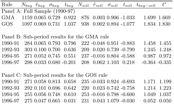
Predictive ability To examine the forecasting ability of the rules, the sig-nals are investigated both individually and together. The results for the pre-dictive ability of the trading rules are reported in Table 5. Both rules display some evidence of significant predictive ability as indicated by the t-statistics in the second last column of Table 5. This result is confirmed by the final column in the table which reports the t-statistic based on the [13] market timing test. However, individually the buy and sell signals do not seem to have any significant predictive ability. In addition to this overall significant predictive ability, all the rules issue buy (or sell) signals when the excess re-turns on the market are on average less (or more) volatile as indicated by the volatility of returns following buy (σbuy) and sell (σsell) signals respectively.
12
Table 4.Performance statistics for GA-optimised share market rules
Rule r XR SR tc∗ T T
w/T rw rL M ax D
Panel A: Full Sample (1990-97)
GMA 10.82 2.45 0.37 53 7.36 44.07 1.72 -0.88 -14.10 GOS 11.16 2.91 0.44 62 6.86 45.45 1.92 -0.98 -10.97 Panel B: Sub-period results for the GMA rule
1990-91 12.48 5.91 0.82 99 7.53 40.00 1.87 -0.97 -6.11 1992-93 16.53 3.59 0.62 69 7.44 46.67 2.20 -0.81 -7.64 1994-95 8.02 2.83 0.45 58 7.50 46.67 1.27 -0.78 -5.40 1996-97 5.20 -3.37 -0.46 0 8.53 41.18 1.20 -0.82 -14.31 Panel C: Sub-period results for the GOS rule
1990-91 11.27 4.64 0.65 87 7.03 35.71 2.58 -1.24 -9.35 1992-93 16.36 3.73 0.64 79 6.45 53.85 2.09 -0.87 -9.10 1994-95 8.35 3.16 0.51 64 7.00 42.86 1.50 -0.71 -5.67 1996-97 7.01 -1.39 -0.19 3 8.53 47.06 1.31 -0.94 -11.02
The Sharpe ratio (SR) is the ratio of annualised excess returns (XR) to standard deviation. The break-even level of transaction cost is given bytc∗. Trading frequency
T is measured by the average number of trades per year. Tw/T represents the
proportion of trades that yield positive excess returns. The average excess return on winning and losing trades is given by rw and rL respectively. The maximum
drawdownM ax Drepresents the largest drop in cumulative excess returns.
Table 5. Predictive ability - share market rules
Rule Nbuy rbuy σbuy tbuy Nsell rsell σsell tsell tbuy−sell t∗
Panel A: Full Sample (1990-97)
GMA 1159 0.065 0.729 0.922 876 0.003 0.906 -1.033 1.699 1.669 GOS 1097 0.069 0.731 1.037 938 0.002 0.894 -1.077 1.834 1.830 Panel B: Sub-period results for the GMA rule
1990-91 284 0.065 0.793 0.796 222 -0.048 0.951 -0.883 1.458 1.455 1992-93 303 0.100 0.700 0.636 209 0.020 0.739 -0.799 1.245 1.248 1994-95 271 0.052 0.745 0.551 237 -0.016 0.804 -0.588 0.987 0.972 1996-97 298 0.033 0.680 -0.201 208 0.062 1.103 0.218 -0.364 -0.335 Panel C: Sub-period results for the GOS rule
[image:21.612.152.451.385.563.2]Table 6.Bootstrap p-values
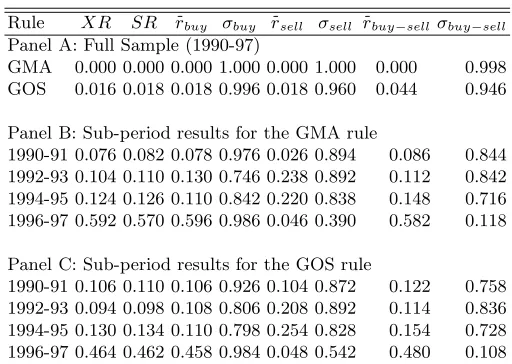
Rule XR SR rbuy σbuy rsell σsell rbuy−sellσbuy−sell
Panel A: Full Sample (1990-97)
GMA 0.000 0.000 0.000 1.000 0.000 1.000 0.000 0.998 GOS 0.016 0.018 0.018 0.996 0.018 0.960 0.044 0.946 Panel B: Sub-period results for the GMA rule
1990-91 0.076 0.082 0.078 0.976 0.026 0.894 0.086 0.844 1992-93 0.104 0.110 0.130 0.746 0.238 0.892 0.112 0.842 1994-95 0.124 0.126 0.110 0.842 0.220 0.838 0.148 0.716 1996-97 0.592 0.570 0.596 0.986 0.046 0.390 0.582 0.118 Panel C: Sub-period results for the GOS rule
1990-91 0.106 0.110 0.106 0.926 0.104 0.872 0.122 0.758 1992-93 0.094 0.098 0.108 0.806 0.208 0.892 0.114 0.836 1994-95 0.130 0.134 0.110 0.798 0.254 0.828 0.154 0.728 1996-97 0.464 0.462 0.458 0.984 0.048 0.542 0.480 0.108 The measures reported in this table are described in Tables 4 and 5
A sub-period analysis of these results indicates that the difference between the average return following buy signals and the average return following sell is no longer significant. This is also true for the market timing test. However, the ability of the rules to buy when volatility in the market is low and sell when volatility is high, appears to be robust across different time periods.
Statistical significance The bootstrap approach outlined in Section 4 is applied to both the trading rule performance and predictive ability results. The simulated p-values for the various measures of performance and pre-dictive ability are given in Table 6. The results for the entire out-of-sample period provide evidence that the rules have significant forecasting power and profitability given that the return series are generated by a random walk pro-cess. However a sub-period analysis shows only weak evidence of significant predictive ability and profitability. In general, these results confirm those reported in Tables 4 and 5.
5.4 Return measurement bias
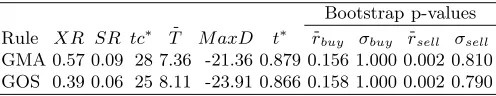
Table 7.Return measurement sensitivity–share market rules
Bootstrap p-values Rule XR SR tc∗ T M axD t∗ r
buy σbuy rsell σsell
GMA 0.57 0.09 28 7.36 -21.36 0.879 0.156 1.000 0.002 0.810 GOS 0.39 0.06 25 8.11 -23.91 0.866 0.158 1.000 0.002 0.790
The performance statistics contained in columns two to seven are described in the notes to Table 4. The last four columns contain bootstrap simulated p-values for the statistics described in Section 4.
As can be seen from Table 7, the rules are still profitable over the out-of-sample test period, although there has been a substantial reduction in performance. Furthermore, there appears to be weak, if any, evidence of pre-dictive ability. However, both rules still retain the property of being in the market when return variability is low and out of the market when return variability is high.
The break-even transaction costs have been reduced to approximately 0.25 percent per trade. This probably lower than the costs faced by most financial institutions. Since stamp duty and taxes are also incurred on all trades, which have been ignored in this evaluation of trading rule performance.13Also
dur-ing volatile periods liquidity costs, as reflected by the bid-ask spread, could increase substantially. Even for large shares this increase could be in the or-der of 0.5 to 1 percent. Thus, there does not appear to be sufficient evidence to conclude that the trading rules are economically profitable.
6
Conclusion
This paper has outlined how a genetic algorithm can be used to optimise technical trading rules and considered an application of this methodology to the Australian share market. The results indicate that there exists some evidence of overall market timing ability, but individual buy and sell signal have only, at best marginal forecasting power for the next days returns. Sur-prisingly, the rules appear to be able to distinguish between periods of low and high volatility. This is an interesting issue which was not investigated in this study, but is left for future research.
Both the GMA and GOS rules were able to outperform the benchmark strategy over the out-of-sample test period, taking into account both trading costs and risks. However, a sub-period analysis of the results indicates that the performance of both rules deteriorates over time. This performance is substantially reduced once the trading rule returns are adjusted for non-synchronous or thin trading.
13
In conclusion, there appears to be some evidence of forecasting ability, but probably little or no evidence of profitability once a reasonable level of trading costs has been considered. Since the break-even costs for these trading rules do not appear to be high enough to exceed realistic trading costs.
References
1. Achelis S. B. (1995) Technical Analysis from A to Z. Probus Publishing, Chicago.
2. Alexander S. S. (1964) Price Movements in Speculative Markets: Trends or Random Walks, No. 2. In: Cootner P. (Ed.) The Random Character of Stock Prices. MIT Press, Cambridge, 338–372
3. Allen F., Karjalainen R. (1999) Using Genetic Algorithms to Find Technical Trading Rules. Journal Finance Economics 51, 245–271
4. Ball R. (1978) Filter Rules: Interpretation of Market Efficiency, Experimental Problems and Australian Evidence. Accounting Education18, 1–17
5. Bauer R. J. Jr. (1994) Genetic Algorithms and Investment Strategies. Wiley Finance Editions, John Wiley and Sons, New York
6. Bessembinder H., Chan K. (1995) The Profitability of Technical Trading Rules in the Asian Stock Markets. Pacific Basin Finance Journal3, 257–284 7. Bessembinder H., Chan K. (1998) Market Efficiency and the Returns to
Tech-nical Analysis. Financial Management27, 5–17
8. Brock W., Lakonishok J., LeBaron B. (1992) Simple Technical Trading Rules and the Stochastic Properties of Stock Returns. Journal of Finance 47, 1731–
1764
9. Brown S., Goetzmann W., Ross S. (1995) Survival. Journal of Finance 50, 853–873
10. Brown S., Goetzmann W., Kumar A. (1998) The Dow Theory: William Pe-ter Hamilton’s Track Record Reconsidered. Working Paper, SPe-tern School of Business, New York University
11. Carter R. B., Van Auken H. E. (1990) Security Analysis and Portfolio Man-agement: A Survey and Analysis. Journal of Portfolio Management, Spring, 81–85
12. Corrado C. J., Lee S. H. (1992) Filter Rule Tests of the Economic Significance of Serial Dependence in Daily Stock Returns. Journal of Financial Research
15, 369–387
13. Cumby R. E., Modest D. M. (1987) Testing for Market Timing Ability: A Framework for Forecast Evaluation. Journal of Financial Economics19, 169– 189
14. Dorsey R. E., Mayer W. J. (1995) Genetic Algorithms for Estimation Prob-lems with Multiple Optima, Nondifferentiability, and Other Irregular Features. Journal of Business and Economic Statistics13, 53–66
15. Efron B. (1979) Bootstrap Methods: Another Look at the Jackknife. Annals of Statistics7, 1–26
16. Fama E., Blume M. (1966) Filter Rules and Stock Market Trading. Journal of Business39, 226–241
18. Holland J. H. (1975) Adaptation in Natural and Artificial Systems. University of Michigan Press, Ann Arbor
19. Huang Y -S. (1995) The Trading Performance of Filter Rules On the Taiwan Stock Exchange. Applied Financial Economics5, 391–395
20. Hudson R., Dempsey M., Keasey K. (1996) A Note on the Weak Form of Efficiency of Capital Markets: The Application of Simple Technical Trading Rules to the U.K. Stock Markets– 1935-1994. Journal of Banking and Finance
20, 1121–1132
21. Koza J. R. (1992) Genetic Programming: On the Programming of Computers By the Means of Natural Selection. MIT Press, Cambridge
22. Levich R. M., Thomas L. R. (1993) The Significance of Technical Trading-Rule Profits in the Foreign Exchange Market: A Bootstrap Approach. Journal of International Money and Finance12, 451–474
23. Lo A. W., MacKinley A. G. (1990) Data Snooping Biases in Tests of Financial Asset Pricing Models. The Review of Financial Studies3, 431–467
24. Maddala G. S., Li H. (1996) Bootstrap Based Tests in Financial Models. In: Maddala G. S., Rao C. R. (Eds.) Handbook of Statistics, V XIV. Elsevier Science, 463–488
25. Malkiel B. (1995) A Random Walk Down Wall Street, 6th edn. W. W. Norton, New York
26. Neely C. J., Weller P., Dittmar R. (1997) Is Technical Analysis in the Foreign Exchange Market Profitable? A Genetic Programming Approach. Journal of Financial Quantitative Analysis32, 405–426
27. Raj M., Thurston D. (1996) Effectiveness of Simple Technical Trading Rules in the Hong Kong Futures Market. Applied Economic Letters3, 33–36 28. Sweeney R. J. (1988) Some New Filter Rule Tests: Methods and Results.
Jour-nal of Financial and Quantitative AJour-nalysis23, 285–301
29. Taylor M. P., Allen H. (1992) The Use of Technical Analysis in the Foreign Exchange Market. Journal of Money and Finance11, 304–314