Active Learning Based Corpus Annotation

Active Learning Based Corpus Annotation

Hongyan Song

1

and Tianfang Yao

2

Shanghai Jiao Tong University

Department of Computer Science and Engineering

Shanghai, China 200240

1_{[email protected]}

2_{[email protected]}

Abstract

Opinion Mining aims to automatically acquire useful opinioned information and knowledge in subjective texts. Research of Chinese Opin-ioned Mining requires the support of annotated corpus for Chinese opinioned-subjective texts. To facilitate the work of corpus annotators, this paper implements an active learning based annotation tool for Chinese opinioned ele-ments which can identify topic, sentiment, and opinion holder in a sentence automatically.

1

Introduction

Opinion Mining is a novel and important re-search topic, aiming to automatically acquire useful opinioned information and knowledge in subjective texts (Liu et al, 2008). This technique has wide and many real world applications, such as e-commerce, business intelligence, informa-tion monitoring, public opinion poll, e-learning, newspaper and publication compilation, and business management. For instance, a typical opinion mining system produces statistical re-sults from online product reviews, which can be used by potential customers when deciding which model to choose, by manufacturers to find out the possible areas of improvement, and by dealers for sales plan evaluation (Yao et al, 2008).

According to Kim and Hovy (2004), an opin-ion is composed of four parts, namely, topic, holder, sentiment, and claim, in which the holder expresses the claim including positive or nega-tive sentiment towards the topic. For example, in the sentence I like this car, I is the holder, like is the positive sentiment, car is the topic, and the whole sentence is the claim.

Research on Chinese opinion mining technol-ogy requires the support of annotated corpus for Chinese opinioned-subjective text. Since the cor-pus includes deep level information related to word segmentation, part-of-speech, syntax,

se-mantics, opinioned elements, and some other information, the finished annotation is very com-plicated. Hence, it is necessary to develop an automatic tool to facilitate the work of annotators so that the efficiency and accuracy of annotation can be improved.

When developing the automatic annotation tool, we find it is most difficult for the tool to annotate opinioned elements automatically. Because unlike other elements such as part-of-speech, and dependency relationship that needed to be anno-tated in the corpus, there is no available tool that can identify opinioned elements automatically. Special classifiers should be constructed to solve this problem.

In traditional supervised learning tasks, train-ing process consumes all the available annotated training instances, so a classifier with high classi-fication accuracy might be constructed. When training a classifier for opinioned elements, it is very expensive and time-consuming to get anno-tated instances. On the other hand, unannoanno-tated instances are abundant in this case, because all the texts in the corpus can be regarded as unan-notated instances before being anunan-notated. This scenario is very appropriate for active learning application. An active learning algorithm picks up the instances which will improve the per-formance of the classifier to the largest extent into the training set, and often produce classifier with higher accuracy using less training instances.

2

Related Work

Common active learning algorithms can be di-vided into two classes, membership query and selective sampling (Dagan and Engelson, 1995). For membership query, algorithm constructs learning instances by itself according to the knowledge learnt, and submits the instances for human processing (Angluin, 1988) (Sammut and Banerji, 1986) (Shapiro, 1982). Although this method has proved high learning efficiency ( Da-gan and Engelson, 1995), it can be applied in fewer scenarios. Since constructing meaningful training instance without the knowledge of target concept is rather difficult. As to selective sam-pling, algorithm picks up training instances which can improve the performance of the classi-fier to the largest extent from a large variety of available instances. Algorithm in this class can be further divided into stream-based algorithm and pool-based algorithm according to how in-stances are saved (Longet al, 2008). For stream-based algorithm (Engelson and Dagon, 1999) (Freund et al, 1997), unannotated instances are submitted to the system successively. All the instances not selected by the algorithms will be discarded. As to pool-based algorithm (Muslea et al, 2006) (McCallum and Nigam, 1998) (Lewis and Gail, 1994), the algorithm choose the most appropriate training instances from all the avail-able instances. Instance not selected might have chance to be picked up in the next round. Though its computational complexity is higher, selective sampling is widely used as an active learning method for no prior knowledge of the target con-cept is required.

Although much research has been made in the field, we found no case which deals with multi-classification problem in active learning. Besides, there is no available method to evaluate the performance of active learning in information extraction.

3

Active Learning Based Corpus

Anno-tation

3.1 System Structure

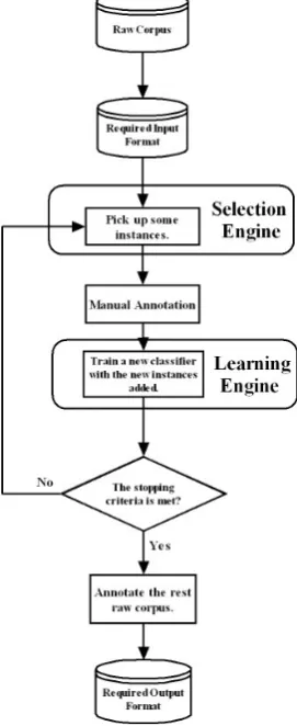
The pool-based active learning algorithm is composed of two main parts: a learning engine and a selecting engine (Figure 1). The learning engine uses instances in the training set to im-prove the performance of the classifier. The se-lecting engine picks up unannotated instances according to preset rules, submits these instances

[image:2.595.352.488.177.509.2]

for human annotation, and incorporates these instances into the training set after the annotation is completed. The learning engine and the select-ing engine work in turns. The performance of the classifier tends to improve with the increasing of the training set size. When the preset condition is met, the training process will finish.

Figure 1 System Workflow

For our active learning based annotation tool, the workflow is as follows.

1. Convert raw texts into the format which the algorithm can deal with.

2. Selecting engine picks up instances which are expected to improve the performance of the classifier to the largest extent.

3. Annotate these instances manually.

4. Learning engine incorporate these anno-tated instances into the training set, and use the new training set to train the classifier.

5. Find out whether the performance of the classifier satisfies the preset standard. If not, go to step 2.

6. Use the classifier to identify the opinioned element in the unannotated dataset.

3.2 Learning Engine

The learning engine maintains the classifier by iteratively training classifiers with new training sets. The classifier adopted determines the up limit of the system performance. We use Support Vector Machine (SVM) (Vapnik, 1995) (Boser et al, 1992) (Chang and Lin, 1992) as the classifier for our system for its high generalization per-formance even with feature vectors of high di-mension and its ability to manage kernel func-tions that map input data to higher dimensional space without increasing computational com-plexity.

3.3 Selecting Engine

In our system, selecting engine picks up in-stances for human annotation, and puts the anno-tated instance into the training set. The strategy adopted when selecting training instance is criti-cal to the overall performance of the active learn-ing algorithm. A good strategy will more likely to produce a classifier with high accuracy from less training instances.

The strategy we adopted here is to choose the instances which the classifier is most unsure about which class they belong to. For a linear bi-classification SVM, these instances are the ones closest to the separating hyper plane. That means, the selecting engine will choose training in-stances according to their geometric diin-stances to the hyper plane. The instance with least distance will be selected as the next instance to be added into the training set while the other instances will be saved for future reference.

The computational complexity of getting the distance between an instance and the hyper plane is low. However, this method can not be applied to SVM with non-linear kernel for geometric distances are meaningless in these cases. We use radial basis function, which is non-linear, as the kernel function in our system for it outperforms linear kernel in the experiment. Hence, we must find another method to pick up training instances.

Non-linear SVM decides the class an in-stance belongs to according to its decision func-tion value.

S

( ) ( )

s

s s s

x

y x

D

y K x x b



˜

¦

&

& & &

(1)

The instance will be classified into one

cer-tain class if , or the other class

if . However, it will be difficult to

clas-sify the instance according to SVM theory if

( )

0

y x

&

!

( )

0

y x

&

( )

0

y x

&

. Hence, we may deduce that SVM is most unsure when classifying an instance with least absolute decision function value.

We define the Predict Value (PV) as the value based on which selecting engine picks up training instances.

For bi-classification SVM, we have PV equals to the absolute decision function value, namely,

PV( )

x

&

y x

( )

&

(2)

Instances with the minimum PV will be selected into the training set before other instances.

For example, if we want to identify all the topics in the sentence,

I like this car very much, but the price is a little bit too high.

ᚒᓛ༑⃶䖭᱅䔺㧘ૉᤚચ䪅㜞ੌὐ㧍

The PV of each instance in the sentences are listed in Table 1. They are calculated from the decision function of the SVM gained from the last round of iteration.

Instances PV

ݺ I 0.260306643320642

ৰ very 0.553855024703612

໛㣴 like 0.427269428974918

㪤 this 0.031682276068012

ཱི type 0.366598504697780

剐 car 0.095961213527654

Δ 0.178633448748979

܀ਢ but 0.092571306234562

᪔匷 price 0.052164989563922

೏ high 0.539913276317129

Ա (auxiliary word) 0.458036102580422

㭠 a little bit 0.439936293288062

Μ 0.375263535139242

Table 1 Example of 2-Classification SVM Predict Value

Suppose all the instances in this sentence have not been added into the training set. This

(0.0316), price (0.0521), and but (0.0925) will be selected into the training set successively for they have the minimal PVs.

there are

1

(

1)

2

t t

˜

decision function values in t -classification SVM.

In our system, we need to classify instances into 4 classes, namely, topic, holder, sentiment

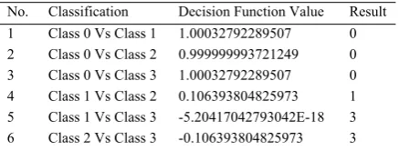
andother. So a 4-classification SVM is adopted. Suppose for an instance, we get 6 Decision Func-tion Values from 6 bi-classificaFunc-tion SVMs as in Table 2.

No. Classification Decision Function Value Result

1 Class 0 Vs Class 1 1.00032792289507 0

2 Class 0 Vs Class 2 0.999999993721249 0

3 Class 0 Vs Class 3 1.00032792289507 0

4 Class 1 Vs Class 2 0.106393804825973 1

5 Class 1 Vs Class 3 -5.20417042793042E-18 3

[image:4.595.72.291.203.286.2]

6 Class 2 Vs Class 3 -0.106393804825973 3

Table 2 Example of 4-Classification SVM Decision Process

For each bi-classification SVM, the class in-stance belongs to is determined by whether the decision function value is greater than or less than zero. The instance in Table 2 belongs to Class 0 since there 3 votes out of 6 votes for Class 0. When deciding which class an instance belongs to, only the decision function values from bi-classification SVMs with correct votes will work on the certainty of the final result. Hence, we define Predict Value for multi-classification SVMs as the arithmetic mean value of the absolute decision function value of every bi-classification SVM with correct vote,

^

t 1, bi classification SVMs with correct votes

1

( ) y ( )

k

t t `

x x

k 

¦

&

39 &

ir

(3)

For the instance in Table2, the value is calculated from the decision function values from bi-classification SVMs numbered 1, 2, and 3.

3.4 Experiments

To prove the validity of active learning algorithm and find out the relations between the perform-ance of the classifiers and the way the classifiers are trained, we carried out batches of experi-ments.

In most information extraction tasks, a word and its context are considered a learning sample, and encoded as feature vectors. In our experi-ments, context data includes the part-of-speech tag, dependency relation, word semantic mean-ing, and word disambiguation information of the

word being classified, its neighboring words and its parent word in dependency grammar. Part-of-speech tag and dependency relation are common features for Chinese Natural Language Process-ing (NLP) tasks1. We get word semantic mean-ing from HowNet, which is an online common-sense knowledge base unveiling inter-conceptual relations and inter-attribute relations of concepts as connoting in lexicons of the Chinese and the English equivalents (Zhendong Dong and Qiang Dong, 1999). Given an occurrence of a word in natural language text, word sense disambiguation is the process of identifying which sense of the word is intended if the word has a number of dis-tinct senses. According to Song and Yao (2009), this information may help in Chinese NLP tasks such as topic identification.

Lack of explicit boundary between training instances and testing instances is a great differ-ence between common machine learning algo-rithm and learning algoalgo-rithm designed for corpus annotation. For common machine learning algo-rithm such as human face recognition, the quan-tity of training instances is limited while the test-ing instances could be infinite. It is unnecessary and impossible to annotate all the testing in-stances. However, when annotating a corpus, all the texts need to be annotated are decided be-forehand. Although tools automated part of the annotation process, the results still need to be reviewed for several times to ensure the quality of annotation. That means in an annotation sce-nario, all the data to be processed are available during the training stage.

The raw texts used in our experiments are taken from forums of chinacars.com. These texts include explicit subjective opinion and informal network language, which are necessary for opin-ion mining research. Most of them are comments composed of one or more sentences on certain type of vehicle. The detailed opinion elements distributions are showed in table 3.

We use all the texts as testing data set and a subset of it as a training data set. First of all, we pick up 10 instances for each class, and train a simple classification model with them. Then, the baseline system picks up k instances in sequence and adds them into the training data set to train a new classification model iteratively until the training data set is as large as the testing data set,

1

while the active learning system picks up in-stances according to the strategy in Chapter 3.3.

Type No. of Instances

[image:5.595.302.536.78.175.2]

Topic 638 Sentiment 769 Holder 46 Other 1500 Total 2953

Table 3 Detailed Information of the Data Set

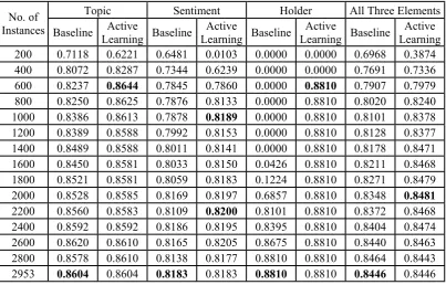
[image:5.595.301.538.82.296.2]

We use three bi-classification model to test the performance of the active learning system on topic, sentiment, and holder identification sepa-rately and a four-classification model to identify the three opinion elements simultaneously. The results of the experiments are illustrated in Fig-ure 2, 3, 4, and 5 respectively. Table 4, 5, and 6 provide the detailed F-measure trends while dif-ferent numbers of instances are added into the training data set in each rounds. For each ex-periment, we try to compare the performances when we add different number of instances into the training data set in each round of iteration.

Figure 2 Topic Identification

Figure 3 Sentiment Identification

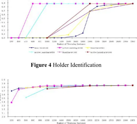
Figure 4 Holder Identification

Figure 5 All Opinion Elements Identification

As are illustrated in the figures, the active learning system can always achieve better or at least no worse performance than baseline system. For example, when adding 200 instances in each round for topic identification task (Figure2 and Table 4), the active learning system reaches its peak value in F-measure (0.8644) with only 600 training instances. This F-measure value is even higher than the value the baseline system get (0.8604) after taking all the 2953 training in-stances.

The active learning system outperforms the baseline system greatly especially when dealing with unbalanced data set (Figure 4 and Table 4). In opinion holder identification task, the baseline system can not find any holder until 1600 train-ing instances are taken while the active learntrain-ing system reaches its peak F-measure value (0.8810) with only 600 training instances. That means when using active learning algorithm, it is possi-ble for us to save some time for optimizing the parameters when dealing with unbalanced data.

[image:5.595.62.293.379.623.2]

4

Evaluation of Active Learning

Algo-rithm

For active learning algorithm based on member-ship query, its training process will probably take longer time by the time the optimum classier is found, since the training process consists of

sev-eral rounds of iteration. At the beginning of the iteration, the classification speed of the model is much faster due to less training instances are used and the model is simple. With more and more training instances are added into the train-ing data set, the model will become more com-plex and more time will be needed for

classifica-ʳ

Topic Sentiment Holder All Three Elements No. of

Instances Baseline Active

Learning Baseline

Active

Learning Baseline

Active

Learning Baseline

Active Learning 200 0.7118 0.6221 0.6481 0.0103 0.0000 0.0000 0.6968 0.3874 400 0.8072 0.8287 0.7344 0.6239 0.0000 0.0000 0.7691 0.7336 600 0.8237 0.8644 0.7845 0.7860 0.0000 0.8810 0.7907 0.7979 800 0.8250 0.8625 0.7876 0.8133 0.0000 0.8810 0.8020 0.8240 1000 0.8386 0.8613 0.7878 0.8189 0.0000 0.8810 0.8101 0.8378 1200 0.8389 0.8588 0.7992 0.8153 0.0000 0.8810 0.8128 0.8377 1400 0.8489 0.8588 0.8011 0.8141 0.0000 0.8810 0.8178 0.8471 1600 0.8450 0.8581 0.8033 0.8150 0.0426 0.8810 0.8211 0.8468 1800 0.8521 0.8581 0.8059 0.8183 0.1224 0.8810 0.8271 0.8479 2000 0.8528 0.8585 0.8169 0.8197 0.6857 0.8810 0.8348 0.8481

[image:6.595.97.501.186.444.2]

2200 0.8560 0.8583 0.8109 0.8200 0.8101 0.8810 0.8372 0.8468 2400 0.8592 0.8592 0.8186 0.8195 0.8395 0.8810 0.8404 0.8474 2600 0.8620 0.8610 0.8165 0.8205 0.8675 0.8810 0.8440 0.8463 2800 0.8578 0.8610 0.8138 0.8177 0.8810 0.8810 0.8464 0.8443 2953 0.8604 0.8604 0.8183 0.8183 0.8810 0.8810 0.8446 0.8446

Table 4 F-measure Trends when k=200

Topic Sentiment Holder All Three Elements No. of

Instances Baseline Active

Learning Baseline

Active

Learning Baseline

Active

Learning Baseline

Active Learning 500 0.8198 0.7730 0.7616 0.1369 0.0000 0.0000 0.7831 0.5173 1000 0.8386 0.8508 0.7878 0.7566 0.0000 0.8837 0.8101 0.7776 1500 0.8468 0.8592 0.8039 0.8175 0.0833 0.8810 0.8194 0.8398 2000 0.8528 0.8610 0.8169 0.8183 0.6857 0.8810 0.8348 0.8484

2500 0.8626 0.8583 0.8168 0.8205 0.8395 0.8810 0.8427 0.8463 2953 0.8604 0.8604 0.8183 0.8183 0.8810 0.8810 0.8446 0.8446

[image:6.595.97.502.488.615.2]

Table 5 F-measure Trends when k=500

Topic Sentiment Holder All Three Elements No. of

Instances Baseline Active

Learning Baseline

Active

Learning Baseline

Active

Learning Baseline

Active Learning 1000 0.8386 0.8335 0.7878 0.3514 0.0000 0.0000 0.8101 0.7534 2000 0.8528 0.8581 0.8169 0.8170 0.6857 0.8810 0.8348 0.8376 2953 0.8604 0.8604 0.8183 0.8183 0.8810 0.8810 0.8446 0.8446

[image:6.595.94.502.658.745.2]

tion. On account of the features of active learn-ing algorithm, we believe it is necessary to find a way to balance the performance of the classifier and the time it take in training process for a thor-ough evaluation of the algorithm.

We define the measurement for time as:

k

T

C

(4)

whereC is the number of all the possible training instances available, k is the number of training instances added into the training data set in each round of iteration. T is the approximate value of the inverse ratio of the time it takes for training process.T will have a greater value if the training process takes less time. Its range is (0, 1] just similar to F-measure.

We define the measurement for the training instances used as:

(1

n

)

K

C

(5)

where n is the number of the training instances actually used. K will have a greater value if less training instances are used in the training process. The range of K is [0, 1).

To judge the overall performance of an active learning algorithm, we consider the F-measure (F) of the classifier, the time it takes during the training process, and the training instances used. We define the Active Learning Performance (ALP) as the harmonic mean of the three aspects:

1

( )

(6)

( ) ( )

ALP

K F T

F k C n

F C k k C n F C C n

D E J

D E J

˜ ˜

˜ ˜ ˜ ˜ ˜ ˜

where

D E J

+ + =1

, and

D E J

, , 

> @

0,1 . They are the weights for the three measurements. The greater the value of a certain weight is, the more important the measurement is in the overall per-formance. The greater the value of the ALP is, the better the performance of the active learning algorithm. For instance, when training a classi-fier for sentiment identification using active learning algorithm, we get a classifier with F-measure of 0.8189 using 1000 training instances and a classifier with F-measure of 0.8200 using 2200 training instances (Table 4).

Sup-pose

= = =

1

3

D E J

, we calculate the value of ALP

for the two cases according to equation (6) and get 0.1714 and 0.1507 as results respectively. That means a people with no preference among F-measure, the number of training instances adopted and the time used during training proc-ess will choose to get a classifier with lproc-ess train-ing instances, less traintrain-ing time and less F-measure value.

5

Conclusion

This paper experimentally demonstrates the va-lidity of active learning algorithm when used for opinioned elements identification and proposed a computational method for overall system per-formance evaluation which consists of F-measure, training time, and number of training instances. According to our tests, active learning algorithm outperforms the base line system in most of the cases especially when fewer in-stances are added into the training data set in each round of iteration. However, the method could extent the training time in a large scale. To balance the pros and cons of active learning algo-rithm, it might be helpful to adjust the number of training instances added in each round dynami-cally in the training process. For instance, add less training instances at the beginning of the training process to ensure a high peak value of F-measure could be achieved and add more train-ing instances later so that time spent on traintrain-ing process could be reduced.

Acknowledgments

The author of this paper would like to thank In-formation Retrieval Lab, Harbin Institute of Technology for providing the tool (LTP) used in experiments. This research was supported by National Natural Science Foundation of China Grant No.60773087.

References

Andrew K. McCallum, Kamal Nigam. 1998. Employ-ing EM in Pool-based Active LearnEmploy-ing for Text Classification. In Proceedings of the 15th Interna-tional Conference on Machine Learning.

Annual Workshop on Computational Learning Theory.

Chih-Chung Chang and Chih-Jen Lin. 2001. LIBSVM: a library for support vector machines. Software available at http://www.csie.ntu.edu.tw/~cjlin/ libsvm

Chih-Wei Hsu and Chih-Jen Lin. 2002. A Compari-son of Methods for Multi-class Support Vector Machines. IEEE Transactions on Neural Networks.

Claude Sammut and Ranan B. Banerji. 1986. Learn-ing Concepts by AskLearn-ing Questions. Machine Learning: An Artificial Intelligence Approach,

1986, 2: 167-191

Dana Angluin. 1988. Queries and Concept Learning.

Machine Learning, 1988, 2(4): 319-342

David D. Lewis, William A. Gail. 1994. A Sequential Algorithm for Training Text Classifiers. In Pro-ceedings of the 17th Annual International ACM SIGIR Conference on Research and Development in Information Retrieval.

Ehud Y. Shapiro. 1982. Algorithmic Program Debug-ging. M.I.T. Press.

Ido Dagan, Sean P. Engelson. 1995. Committee-Based Sampling for Training Probabilistic Classi-fiers. In Proceedings of the International Confer-ence on Machine Learning.

Ion Muslea, Steven Minton, Craig A. Knoblock. 2006. Active Learning with Multiple Views. Journal of Artificial Intelligence Research, 2006, 27(1): 203-233.

Quansheng Liu, Tianfang Yao, Gaohui Huang, Jun Liu, Hongyan Song. 2008. A Survey of Opinion Mining for Texts. Journal of Chinese Information Processing. 2008, 22(6):63-68.

Jun Long, Jianping Yin, En Zhu, and Wentao Zhao. A Survey of Active Learning. 2008. Journal of Com-puter Research and Development, 2008, 45(z1): 300-304.

Shlomo A. Engelson, Ido Dagon. 1999. Committee-based Sample Selection for Probabilistic Classifi-ers. Journal of Artificial Intelligence Research, 1999, 11: 335-360.

Hongyan Song, Jun Liu, Tianfang Yao, Quansheng Liu, Gaohui Huang. 2009. Construction of an An-notated Corpus for Chinese Opinioned-Subjective Texts.Journal of Chinese Information Processing, 2009, 23(2): 123-128.

Hongyan Song and Tianfang Yao. 2009. Improving Chinese Topic Extraction Using Word Sense Dis-ambiguation Information. In Proceedings of the 4th International Conference on Innovative Computing, Information and Control.

Soo-Min Kim and Eduard Hovy. 2004. Determining the Sentiment of Opinions. In Proceedings of the Conference on Computational Linguistics: 1367-1373.

Tianfang Yao, Xiwen Cheng, Feiyu Xu, Hans Uszkoreit, and Rui Wang. 2008. A Survey of Opin-ion Mining for Texts. Journal of Chinese Informa-tion Processing, 2008, 22(3): 71-80.

Vladimir N. Vapnik. 1995. The Nature of Statistical Learning Theory. Springer.

Yoav Freund, H.Sebastian Seung, Eli Shamir, Naftali Tishby. 1997. Selective Sampling Using the Query by Committee Algorithm. Machine Learning, 28(2-3): 133-168