Linear and Nonlinear Model Predictive Control of Quadruple Tank Process

(1)

Linear and Nonlinear Model Predictive Control of

Quadruple Tank Process

P.Srinivasarao

Research scholar Dr.M.G.R.University

Chennai, India

P.Subbaiah, PhD.

Prof of Dhanalaxmi college of Engineering Thambaram

Chennai, India

ABSTRACT

In a multi input and output (MIMO) process mathematical modeling of the physical systems has gained importance due to the complexity of interactions within the system. All the parameters used in a model cannot be determined accurately. The major problem in a multivariable process is that loop interaction can arise and cause difficulty in feedback control design. This problem can be solved using centralized or decentralized controllers. One of the centralized techniques is model predictive control, which can be measured current to predicted future values of outputs. In this paper, model predictive control (MPC) technology for both linear and nonlinear model of quadruple tank process is proposed. It consists of four inter connected water tanks and two pumps as shown in figure 1. A general MPC control is presented, and approaches taken for the different aspects of the calculation are described. It is shown that MPC control is more stable, responsive and robust.

Keywords

MIMO, MPC, Quadruple Tank Process, Robust.

1. INTRODUCTION

The major problem is to solve the control parameters for static as well as dynamic systems using model predictive control (MPC). Here, MPC is a more advanced method to control the predicted output along with tuning the parameters such as prediction and control horizons and control weights. It can handle multivariable processes, difficult multivariable control problems that include inequality constraints [11]. Linear MPC refers to a family of MPC schemes in which linear models are used to predict the system dynamics, even though the dynamics of the closed-loop system is nonlinear due to the presence of constraints [10]. Linear [5] and Nonlinear [6] MPC approaches have found successful applications, especially in the process industries. The process is called the quadruple-tank process and consists of four interconnected water tanks and two pumps. The system is shown in Figure 1. The inputs are the voltages to the two pumps and the outputs are the water levels in the lowertwo tanks. The quadruple-tank process can easily be built by using two double-quadruple-tank processes. The linearized model of the quadruple-tank process has a multivariable zero, which can be located in either the left or the right half-plane by simply changing a valve. Quadruple tank contains transmission zeros, which can vary from left half plane (minimum phase) to right half plane (non-minimum phase) depending on the ratio of the flow to upper and lower tanks.

The step response of the quadruple tank system using MPC with different control values is obtained and compared to the step response of the controlled system using Decoupled control strategy [1] and Comparative study [2].

This paper is organized as follows: section 2 gives description of four tank process. The controller design for four tanks and simulation analysis for stability is explained in 3 & 4. Finally the conclusion is given in 5

2. DESCRITON

OF

FOUR

TANK

PROCESS

Quadruple-tank process consists of four interconnected water tanks and two pumps as shown in Figure 1. The target is to control the level in the lower two tanks with two pumps [3]. The process inputs are v1 and v2 (input voltages to the pumps) and the outputs are

y

₁



k h

_c ₁ and

y

₂



k h

_c ₂ (voltages from level measurement devices). Mass balances and Bernoulli’s law yield the following model:









3

1 1 1 1

1 3 1

1 1 1

2 2 4 2 2

2 4 2

2 2 2

2 2 3 3 3 2 3 3 1 1 4 4 4 1 4 4

2

1

2

1

2  



 





 





 



a

dh

a

k

gh

v

dt

A

dh

a

k

gh

v

dt

A

k

dh

a

gh

v

dt

A

k

dh

a

gh

v

dt

A



(1)

where,



_i is the flow distribution to lower and diagonal upper tank,

A

_i is the cross-section area,

a

_i is the outlet hole cross section and

h

_i is the water level, in tank i respectively. The voltage applied to pump i is

v

_i and the corresponding flow is

k v

_{i i}. The parameters

 

₁, ₂

 

0,1 are determined from how the valves are set prior to an experiment. The flow to tank 1 is

y k v

_{1 1 1} and the flow to tank 4 is



1 

y k v

₁



_{1 1} and similarly for tank 2 and 3. The acceleration of gravity is denoted ‘g’. This typical system has two finite zeros for

 

1, 2 0,1

(2)

[image:2.595.63.257.72.274.2]

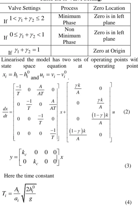
Fig. 1. Diagram for Quadruple Tank Process.

Table 1. For Valve Setting.

Valve Settings Process Zero Location

If

1  



1



2



2

Minimum

Phase

Zero is in left plane

If

0  



1



2



1

Non Minimum

Phase

Zero is in left plane

If



1





2



1

Zero at Origin

Linearised the model has two sets of operating points with state space equation at operating points

0

i i i

x

 

h

and

0

i i i

u

 

v

.









1 1 3 1

1 1 3

2 2

4

2

2 2 4

2 2 3 3 1 1 4 4 1 ₀ 0 0 1 ₀ 0 0 1 1

0 0 0 0

1 1

0 0 0 ₀

k A A T AT k A A T AT dx x u k dt T A k T _A          _ _   _ _   _ _    _ _   _ _   _ _ _{ } _ _  _ _   _ _   _ _  _  _ _ _   _ _     _ _ (2)

0 0 0

c c k y x k     

  ₍₃₎

Here the time constant

0

2

i i i i

A

h

T

a

g



(4)

The dynamics for the process transfer function matrix is

 





























2 2 1 1

1 3 1

1 2 2 2

4 2 2

1

1 1 1

1

1 1 1

c c

sT sT sT

G s

c c

sT sT sT



            _        

 ₍₅₎

3. DESCRIPTION OF MPC

In MPC applications, the output variables are also referred to as controlled variables or CV’s, while the input variables are called as manipulated variables or MV’s. The predictions are made in two types of MPC calculations that are performed at each sampling instant: set-point calculations [5] and control calculations. Inequality constraints as upper and lower limits can be included in either types of calculation [6].

In MPC the set points are typically calculated each time for MIMO process with u input variables and y output variables

The current values of u and y as u(k) and y(k). The objective is to calculate the optimum set point ysp for the next control

calculation (at k+1) and also to determine the corresponding steady-state value of u, usp. This value is used as the set point

for u for the next control calculation.

A general, linear steady-state process model can be written as [10]

y K u

  

(6)

Where K the steady-state is gain matrix and  u, ydenotes steady-state changes in u and y it is convenient define



u

andy as

 

sp

y

yOL k

 



(7)

Here

yOL k

 

is steady-state value of y

 

sp

u

u k

 



(8) To incorporate output feedback, the steady-state model Eqn (6) is modified as

   

y

K u



y k



   

_



_

(9)

3.1 The principle of linear and nonlinear

model predictive control

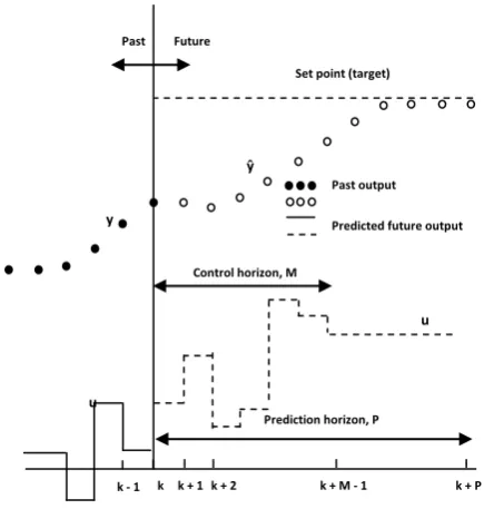
[image:2.595.52.276.318.652.2]

(3)

[image:3.595.52.270.70.299.2]

Fig. 2: Basic principle of Model Predictive Control.

The main point of this optimization problem is to compute a new control input vector,

u k

 

to be fed to the system, and at the same time take the process constraints into consideration.

An MPC algorithm consists of:

Cost Function, Constraint and A Model of the Process.

3.2 Cost Function

The main idea with MPC is that the MPC controller calculates a sequence of future control actions such that the cost function is minimized.

The cost function often used in MPC is like this (a linear quadratic function)[10]:



 



0 0

ˆ

p p N N T T k k

J

y

r

Q y

r

u R u

 







 





(10)

Where:

p

N



Prediction horizon

r



Set point

ˆ

y



Predicted process output

u

 

Predicted change in control value,

 

u

k

u

k



u

k1

QOutput error weight matrix

RControl weight matrix

This works for MIMO systems (Multiple Input and Multiple Outputs) so we are dealing with vectors and matrices.

3.3 Constrains

All physical systems have constraints. Generally, physical constraints like actuator and valve limits, etc and performance constraints like overshoot, settling time, etc. In MPC one normally defines these constraints [10] to minimize inequalities.

Constraints in the outputs:

min max

y

 

y

₍₁₁₎

Constraints in the inputs:

min max

u



   

(12)

min max

u

 

u

(13)

Note:

 

u

k

u

k



u

k1

3.4 Model

The main drawback with MPC is that a model for the process, i.e., a model which describes the input to output behavior of the process, is needed. Mechanistic models derived from conservation laws can be used. Usually, however in practice simply data-driven linear models are used.

In MPC it is assumed that the model represents a state-space model of the form [8]:

 

,

x k



Ax



Bu

 

.

y k



Cx



Du

(14)

We consider the stabilization problem for a class of systems described by the following nonlinear of differential equations [8]:

 

   

, , 0,

 

0 0,

x t A t f x t u t_ _ t x t x

 

0

,

. :

c m c m

x

 

X

R

u

 

U

R

A

R





R

 (15) With the known smooth nonlinear map

f x t u t



_

   

,



_

and the unknown parameter matrix

A t

 

4. SIMULATION ANALYSIS

In this paper, simulation results are compared with [1] and [2] on time based domain using tuning predictive control response, to a step response input. Here, response is plotted for the lower tanks for minimum and non minimum phase at two operating points is studied at p- and p+ of minimum and

non minimum phase [9]. These operating points are at Table.2.

For minimum phase response of linear system with P=10, M=2, no of control interval=1 as shown in Fig. 3 when tuning the parameters the response is shown in Fig.4, here P=10, M=3, no of control interval=0.25.

Table 2. Operating Points.

Operating

Points Units p- p+



0 0



1

,

2

h h

[cm] (12.4, 12.7) (12.6, 13.0)



0 0



3

,

4

h h

[cm] (1.8, 1.4) (4.8, 4.9)



0 0



1

,

2

v v

[V] (1,1) (1, 1)



k k

1

,

2



[cm 3

/Vs] _{(3.33, 3.35)} _{(3.14, 3.29)}



 

1

,

2



(0.7, 0.6) (0.43, 0.34)

k - 1 k k + 1 k + 2 k + M - 1 k + P u

Prediction horizon, P y

ŷ

u Control horizon, M

Set point (target) Future

Past

Past output

Predicted future output

Past control action

[image:3.595.310.536.612.744.2]

(4)

Fig.3 Output response with specified input

For non minimum phase response of linear system with P=10, M=2, no of control interval=1 as shown in Fig. 5. When tune parameters the response is shown in Fig.6, here P=10, M=3, no of control interval=0.25, along delay of 1second.

(5)

For minimum phase response of linear system without applied input

u

2

is shown at Fig. 7, similarly response obtained without input

u

1

is shown at Fig.8.

Fig.7 Output response with specified input u1

Similarly for non minimum phase response of linear system without applied input

u

2

as shown in Fig. 9, similarly response obtained without input

u

1

as shown in Fig.10.

Fig.10 output response with specified input u2

(6)

[image:6.595.54.285.70.433.2]

Fig. 11 output response with specified input

Fig.12Output response with specified input

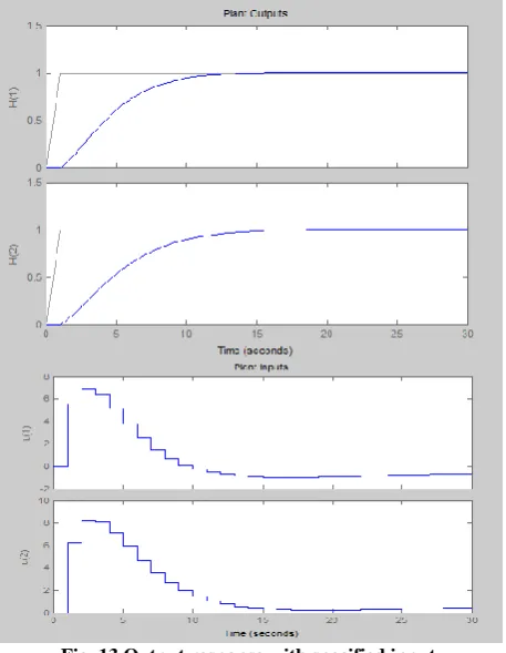
[image:6.595.317.544.128.727.2]

For non minimum phase response of non linear system with P=10, M=2, no of control interval=1, along delay of 1second is shown in Fig. 13, when tune parameters the response is show in Fig. 14, here P=10, M=3, no of control interval = 0.25.

Fig. 13 Output response with specified input

[image:6.595.316.545.131.426.2]

(7)

5. CONCLUSION

The design procedure for MPC controller for Quadruple tank process has been proposed in this paper. The step response for process is compared with the results obtained in references listed as paper1 and paper 2 for both minimum and non minimum phase of linear and nonlinear system. It is observed that linear and nonlinear process with different controller parameters offers stable response for step input. Nonlinear system exhibits stable response without overshoots for minimum and non minimum phase. Similarly linear systems also exhibit stable response without overshoot for certain tuned controller parameters. Response of linear system for the lower two tanks, when absence of one input, one of them exhibits stable response for set point of respective step input. Remaining tank exhibits slit stable response not up to set point. Non minimum phase system has a transmission zero on right plane still exhibits stable response without any compensation for linear and non linear system. MPC is a more advanced technique to handle multivariable parameters. Finally, all transient and steady state responses have been obtained in all cases.

6. REFERENCES

[1] P. Srinivasarao and Dr. P. Subbaiah, “Decoupled control strategy for quadruple tank process,” CIIT International Journal of Programmable Circuit and System, Vol. 4, No. 6, pp. 287-296, May 2012.

[2] P. Srinivasarao and Dr. P. Subbaiah, “Comparative study for Quadruple Tank Process with Coefficient Diagram Method,” IFRSA International Journal of Electronics Circuits and System, Vol. 1, Issue 2, pp. 90-99, July 2012.

[3] K. H. Johansson, “The Quadruple-Tank Process: A Multivariable Laboratory Process with an Adjustable Zero,” IEEE Transactions on Control Systems Technology, pp. 456–465, 2000.

[4] Qamar Saeed, Vali Uddin and Reza Katebi,

“Multivariable Predictive PID Control for Quadruple Tank,” World Academy of Science, Engineering and Technology,2010.

[5] M. Alamir, G. Bornard, " Stability of a truncated infinite constrained receding horizon scheme: the general discrete nonlinear case,” Elsevier Science Ltd , Vol. 31, No. 9, pp. 1353-1356, Sep 1995.

[6] Zoltan K.Nagy Richard D.Braatz, “Roboust Nonlinear Model Predictive Control of Batch Processses”, AIChe Journal, Vol. 49 No.7, July 2003.

[7] M. J. Lengare, R. H. Chile, L. M. Waghmare and Bhavesh Parmar, “Auto Tuning of PID Controller for MIMO Processes,” World Academy of Science, Engineering and Technology, 2008.

[8] Sergey Edward Lyshevski, Control system theory with Engineering Applications, Jaico Publishers, 2003.

[9] Ashish Tewari, Modern Conrol Design with MATLAB and SIMULINK, John Willy & Sons, Ltd, 2009.

[10] Dale E. Seborg,Thomas F. Edgar and Duncan A.Mellichamp , Process Dynamics and Control, John Willy & Sons, Ltd, 2006.

[11] B.Wayane Bequette , Process Control Modeling, Design and Simulation, Prentice Hall,2003.

AUTHOR’S PROFILE

P. Srinivasarao working as Associate Professor in VITS Group of Institutions, Sontyam, Visakhapatnam. Completed M.Tech from COE Pune, Ph.D Scholar, Dr. M.G..R. University.