An Improved Fast Watershed Algorithm based on finding the Shortest Paths with Breadth First Search

(1)

An Improved Fast Watershed Algorithm based on

finding the Shortest Paths with Breadth First Search

Suphalakshmi. A

Anandhakumar P

Department of IT, Paavai Engineering college,

Namakkal, TamilNadu

,

Department of IT, Madras Institute of

Technology Campus, Anna University Chennai

,

ABSTRACT

A watershed based on rainfall simulation is a proven technique for image segmentation. The only problem associated with it is the path regularization for pixels in the plateau. As the existing methods employ sequential techniques, the complexity of the algorithms remains high due to repetitive scanning of pixels. We propose an iterative method for finding the shortest and steepest path based on Breadth first search (BFS), which addresses the path regularization problem eliminating the repetitive scans. Experiments show, that the proposed algorithm significantly reduces the running time without compensating the performance when compared with the fastest known algorithm.

General Terms

Fast watersheds, Image segmentation, Breadth First search, shortest path, path regularization.

1. INTRODUCTION

Image segmentation is a fundamental problem in image analysis. The segmentation process can rely both on the uniformity of features within the regions or on edge evidence. The watershed transform from mathematical morphology is a powerful region based image segmentation algorithm [4]. It has been applied in various fields of images segmentation such as medical image segmentation [24] [28], Remote sensor images [24], cell image segmentation [25], CCD infrared image segmentation [23] and for the segmentation of bubble images [18].

Idea of watershed algorithm was developed from the field of topography. If we consider the analogy of a landscape and rain, water will find the swiftest descent path until it reaches some lake or sea, we can envisage lakes and seas correspond to regional minima [7]. The landscape can be completely partitioned into regions which draw water to a particular sea or lake. These regions are influence zones of the regional minima in an image which forms catchment basin. Watersheds, also called watershed lines, separate catchment basins.

From the literature we can find various flavours of watershed algorithms based on markers [24], graphs and graph cuts [19], level sets [20] and a number of improved versions from the references [25], [27], [28] and [29]. Watersheds algorithm was also extended to 3D space by Lee Seng yeong et. Al. [26]. Though there are lot of variations and combinations with other methods, watershed still remain in research to improve either its time complexity, reducing the problem of over segmentation, and solving the path regularization. We, in this paper address all the three problems of watershed with our proposed algorithm.

1.1 Watershed Segmentation

Gradient of an image resembles a topographic surface. Pixels having the highest gradient magnitude intensities (GMI) correspond to watershed lines, which represent the region boundaries. Water placed on any pixel enclosed by a common watershed line flows downhill to a common local intensity minimum (LIM). Pixels draining to a common minimum form a catchment basin, which represents a segment.

There are two conceptually distinct methods for computing watershed transform in digital images. The traditional watershed algorithm is usually implemented by simulating a flooding through immersion. The immersion simulation process starts with piercing holes in each minima (LIM), then this surface is gradually immersed into water. Starting from the minima of lowest altitude, water progressively fills different catchment basins. When water coming from different minima is about to merge, dams are built to prevent intermingle [3] [7]. At the end of the flooding process, each catchment basin is separated from the other by dams.

Though morphological watersheds (immersion based) [2] [7] are proven to be powerful image segmentation algorithm, they entail a common problem, which is oversegmentation of smaller regions. This is mainly due to construction of watershed lines to limit flooding [7, 3]. Fig.. 1, illustrates over segmentation problem of morphological watersheds in one dimensional space.

Even though there are two regional minima, morphological watershed constructs only one catchment basin. Moreover morphological watersheds also create thick watershed lines, but segmentation results are desirable to have lines which never have a width greater than the minimum resolution in the digital image (usually one pixel).

(2)

[image:2.595.74.274.81.227.2]

Fig. 1. Illustration of watershed line and oversegmentation of watersheds based on flooding in one-dimensional case.

In this approach, no pixel will explicitly belong to a watershed line, because every pixel is labelled as belonging to a certain basin. The lines will therefore be formed by the edges of the pixels that separate the different basins. Since each regional minimum has its own catchment basin, oversegmentation never occurs in rainfall based methods. Fig.. 2 shows construction of catchment basins by rainfall simulation.

Fig. 2. Creation of catchment basins through rainfall simulation.

[image:2.595.101.247.344.448.2]

This method has been implemented in Ref. [8], and improved in Refs. [1, 3, 9, 14]. There also exist other studies focusing on hardware adaptation [15] [27], and parallel processing [15,16].

Nevertheless, rainfall based methods can create watersheds only if every pixel in the image has a steepest neighbour (lower gray level). In images there exist plateaus where pixels are at same gray level. For such pixels path cannot be computed directly. Many algorithms were proposed to solve the path regularisation problem. Bieniek et .Al [1] proposed a method based on geometry of the plateau which computed path for plateau pixels effectively using connected components.

Han Sun et al [3] simplified the computation structure with the help of chain codes to represent connected component which were used by Bieniek for arrowing. In both of the algorithms image is explored five times allowing a running time lower than the fastest at that moment [2,17]. Victor et al [9] enhanced Han Sun‟s algorithm by limiting the necessary neighbouring operations to compute the transform to the outmost and achieved results using three scans, thus decreasing the running time obtained by Sun [3] and Bieniek [1]. Rambabu et. Al [27] has proposed a hill climbing method which also produces a linear time complexity. But existing methods use sequential approach which limited them from achieving maximum efficiency.

In this paper we propose an iterative method to solve path regularisation problem. The proposed algorithm can compute the watershed transform more effectively than existing methods and is capable of producing results with lower running time than current approaches. We demonstrate both assertions throughout this paper supported by several examples.

The paper is organized as follows; Section 1 being the preamble, section 2 describes the necessary definitions for creating watersheds. Section 3 details the problems with existing algorithms using sequential approach to solve path regularisation. The proposed algorithm is elaborated in section 4. In section 5 we display the results and analyse the time complexity of our algorithm with the existing methods, finally, we conclude in section 6.

2. DEFINITION AND PROPERTIES

OF THE WATERSHEDS

In this section we describe the basic definitions and properties of watershed based on rainfall simulation which are used throughout this paper.

Let us consider a two-dimensional gray scale image f whose definition domain is denoted DI ⊂ ℤ2. f is supposed to take discrete (gray) values in a given range [0, N], N being an arbitrary positive integer.

Let G denote a square grid and ‘p’ denotes a pixel in 𝐺 ∈ ℤ2_{𝑥 ℤ}2_{. Path of a water drop can be expressed as follows,} Definition 1: A path „𝒫‟ of length L between two pixels‘𝑎’ and ‘𝑏’ in image 𝑓 is an (𝐿 + 1) ordered pair of pixels starting from ‘𝑎’ and ending in‘𝑏’.

𝒫 a ,b = p0, p1, … , pL−1, pL | p0= a, pl= b ∶

∀ pi∈ NG pi−1 , i = 1 … l (1)

Where, 𝑁𝐺(𝑝) denotes the set of the neighbouring pixels of pixel‘𝑝’, with respect to 𝐺

NG(p) = {p′∈ Z2, (p, p′) ∈ G} (2)

It is important to define the type of connectivity for the neighbourhood operation. Typically either four connectivity (every pixel is connected with neighbours in vertical and horizontal direction) or 8 connectivity (diagonal pixels are also included) is used. We assume 8 connectivity throughout the paper, as it increases neighbourhood operation.

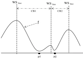
In terrain surface a water drop will flow along a steepest descent path until it reaches minimum [1, 3, 4]. A digital image is analogous to a terrain surface in which, pixels with higher gray level form hills and those with lower gray level form lakes. Fig. 3 pictures the topology simulation of a sample image.

WSline

ƒ

µi µj WSline WSline

CB1 CB2

WS _line

ƒ

WS line

µi µj

(3)

(a)

(b)

[image:3.595.80.298.62.523.2]

(c)

Fig. 3. Topology structure of gradient image. (a) Sample gray scale image. (b) Sobel’s Gradient magnitude of Fig. 3.a. (c) 3d representation of

Fig. 3.b.

In rainfall based watersheds every path starts from pixel at higher altitude and end in a pixel at lowest altitude. A regional minimum is a pixel having gray level value smaller than any other pixels in the region [3,8-11]. Hence, a steepest descending path SP(p,μ) can be defined as below,

Definition 3: Steepest descent path from a pixel ‘𝑝’ to minimum ‘𝜇’ is a series of connected pixels originating from‘𝑝’; such that every descendent pixel in SP is strictly smaller (low gray value) than its predecessor.

SP(p,μ)= 𝒫(p,μ)∶ pi< pi−1 where i = 0,1, … , L. (3)

Suppose there are n regional minima

𝜇1, 𝜇2, 𝜇3, … , 𝜇𝑛−1, 𝜇𝑛 the catchment basin is defined as: Definition 4: The catchment basin 𝐶𝐵𝑖 associated with a regional minimum 𝜇𝑖 is the set of pixels p of DI such that a

water drop falling at 𝑝 flows down along the relief, following

a certain descending path called the downstream of 𝑝 [2,13], and eventually reaches M.

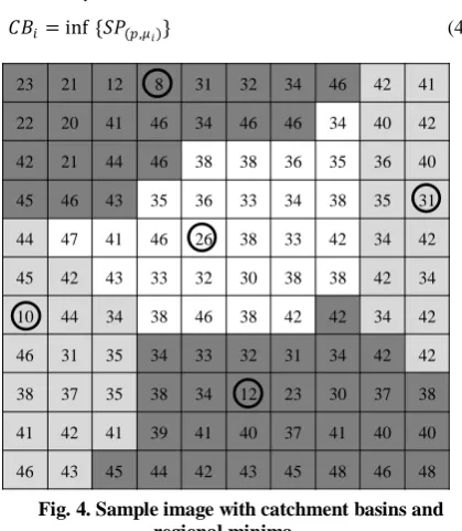
[image:3.595.326.536.92.333.2]

𝐶𝐵𝑖 = inf {𝑆𝑃(𝑝,𝜇𝑖)} (4)

Fig. 4. Sample image with catchment basins and regional minima.

Therefore a catchment basin is a domain in an image, In Fig. 4, the shaded regions are the catchment basins to their corresponding regional minima which are encircled.

Definition 5: The geodesic distance between two pixels p and q belonging to a certain domain CB in an image is the minimum length of any path from p to q without leaving the domain CB.

𝐺𝐷 𝑝, 𝑞 = inf S𝒫(𝑝,𝑞)| 𝑝, 𝑞 ∈ 𝐶𝐵𝑖 (5)

Following is another definition of catchment basin based on minimum geodesic distance,

Definition 6: A catchment basin 𝐶𝐵𝑖 associated with a regional 𝜇𝑖 is a set of pixels closer to 𝜇𝑖 than to any other regional minima 𝜇𝑗.

𝐶𝐵𝑖 = 𝑝 ∶ 𝐺𝐷 𝑝, 𝜇𝑖 < 𝐺𝐷 𝑝, 𝜇𝑗 (6)

3. PROBLEM FORMULATION

Many images have regions where pixels have the same gray level. These plateaus of pixels pose a problem when they do not form regional minima [1-3]. Since there are no neighbour with lower gray level, computation of steepest descent path cannot be done as given by definition 3. Solution to this problem is based on the geometry of the plateau. Pixels at the boundary of non minimal plateau will have a steepest descent path [8] and will be associated with a catchment basin. By calculating the geodesic distance between edge pixels and non edge pixels, steepest descending path can be assigned to the edge pixel whose cost function is low.

In existing methods [1-3] this solution is achieved by dividing the plateau into two groups:

1. Descending edge points of plateau: this group consists of every point of the plateau that has a neighbour with a gray level less than its gray level.

23 21 12 8 31 32 34 46 42 41

22 20 41 46 34 46 46 34 40 42

42 21 44 46 38 38 36 35 36 40

45 46 43 35 36 33 34 38 35 31

44 47 41 46 26 38 33 42 34 42

45 42 43 33 32 30 38 38 42 34

10 44 34 38 46 38 42 42 34 42

46 31 35 34 33 32 31 34 42 42

38 37 35 38 34 12 23 30 37 38

41 42 41 39 41 40 37 41 40 40

(4)

2. Inner points of plateau: this group consists of every point of the plateau whose neighbours have gray levels of equal or higher value than its gray level.

Subsequently, the geodesic distance of an inner point of the plateau to all edge points is calculated having the plateau as domain [1, 3, and 9]. Steepest path is formed to edge point whose geodesic distance is low. However, this sequential method for computing the steepest path requires finding all edge pixels in the plateau, which can be achieved only if the image is scanned at least once [1], thus imposing a mandatory complexity O(N), where N is the number of pixels in the image.

Furthermore, if there are 𝑚 pixels in a plateau of which 𝑚1

and 𝑚2 pixels belong to edge and inner points respectively, then computing steepest path for all pixels in 𝑚2 is the Cartesian product of 𝑚1 and 𝑚2. Hence, if the size of plateau is large or number of plateaus is high or both, then these algorithms suffer high execution time.

4. PROPOSED ALGORITHM

An edge pixel with low cost implies that it can be reached more swiftly than any other edge pixel in plateau. Therefore, instead of computing geodesic distance to all edge points, an iterative approach can be adopted to search foremost edge pixel and assign the steepest path to corresponding edge pixel. Hence, time spent in finding all edge pixels and computing geodesic distance between them can be eliminated. Since a Breadth First Search (BFS) algorithm processes all pixels at the same distance from the current pixel before moving to next level, incremental geodesic search can be achieved. BFS can be adopted to search the foremost edge pixel and assign the steepest path to the corresponding pixel.

4.1 Description of Algorithm

The proposed algorithm has two major steps: First is to arrow complete image function and second is to label the regional minima and propagate the labels along the image via arrowing. Arrowing process is represented with the help of chain codes [12]. Fig. 4 illustrates chain code values for the direction to which current pixel points. Fig. 4.b is the mirror image of Fig. 4.a, which represents the value a neighbourhood pixel must possess when it points to current pixel.

Fig. 5. (a) Chain code (b) Modified chain code (From reference [3])

[image:4.595.317.546.73.257.2]

In Fig. 6, the path from the pixel 49 at position (10, 4) to pixel 14 at position (7, 8) is represented by arrows; its corresponding chain code representation is 001211. Mirror image simplifies the process of tracing the arrows during labelling step. Regional minima are differentiated by assigning a special chain code value 8.

Fig. 6. Example of steepest descending path. Solid lines represent the steepest descending path that originates

from point (10, 4) until a minimum situated in (7, 8). Regional minima are encircled.

4.2 Arrowing step

The proposed algorithm scans image sequentially and computes steepest descending path to all pixels having at least one lower neighbour. Regional minima are assigned a special chain code values and their position is stored in a queue which will be used in labelling step. For pixels belonging to lower complete image, the algorithm initiates a breadth first search algorithm. Fig. 7 exemplifies the arrowing process with the proposed algorithm.

Fig. 7. Arrowing process of the proposed algorithm

(a)

3 2

7 6

0 4

5

1 7 6

3 2

4 0

1

5

(a) (b)

20 14 17 28 26 19 18 15 21 20

15 13 15 21 20 15 15 17 18 17

17 20 22 25 23 15 15 15 17 17

29 35 37 40 35 27 25 22 16 17

29 34 34 31 28 27 28 28 26 22

25 13 14 15 17 24 23 16 27 30

49 40 44 16 16 16 15 14 23 30

40 40 40 47 22 17 17 19 22 29

40 40 40 40 32 27 19 21 23 25

11 40 40 49 29 24 22 22 21 21

Is pixel belongs to

plateau

Label as plateau pixel Is pixel a

regional minima?

Initiate BFS

Assign shortest steepest path Label as normal

pixel

Label as regional minima Assign to the

lowest neighbour

Pixel Input

image

yes No

No yes

46 46 38 29 42

38 29 29 38 38

38 46 38 42 42

34 34 34 34 34

[image:4.595.315.564.412.611.2] [image:4.595.77.269.529.628.2]

(5)

(b)

(c)

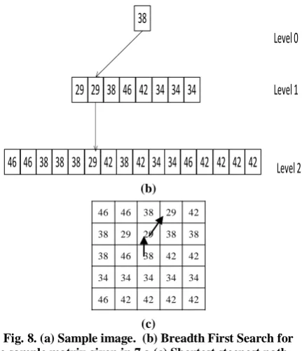
Fig. 8. (a) Sample image. (b) Breadth First Search for the sample matrix given in 7.a (c) Shortest steepest path

for the sample matrix

As mentioned earlier we use 8 pixel connectivity, In an eight connectivity, all the 8 neighbouring pixels are pushed in to the queue in raster scanning order.

Let p be the pixel to which steepest path cannot be computed directly. The algorithm initiates a BFS with p as root node as level 0. The BFS algorithm scans neighbouring pixels and inserts them in a queue when value of neighbouring pixel is less than or equal to root node. The process stops when a minimum is found after scanning all the pixels in current level or next level is out of the plateau. When the BFS terminates we can encounter one of the following cases:

1. A minimum is obtained. 2. No minimum is obtained

Computation of steepest descending path for two cases is done as follows:

Case one: By definition 6, path to the node with least value should be assigned as steepest path. All pixels belonging to non minimal plateaus will form case one.

Case two: only minimal plateaus will create case two. Steepest path is assigned to any of the leaf nodes and the leaf node is represented as regional minimum.

4.3 Labelling of Catchment Basins

Once arrowing of the function ℱ is completed, catchment basins can be labelled following the arrows. Each regional minima identified in arrowing step is put into a queue (one at a time). Until the queue is not empty, an element is dequeued and its neighbouring chain code values are compared with modified chain codes and the following operations are performed:

1. Value of dequeued element is assigned a label (Normally gray value of current regional minima) 2. All neighbouring pixels whose chain code values

match with modified chain codes are enqueued back

4.3.1 Algorithm Description

The following are the description of elements and operations used in the algorithm,

Input image : f

Output image : w

Neighbour of pixel p at distance L : NL(p)

Inserting an element in a queue : Enqueue(q)

Removing an element from queue : dequeue(q)

Current pixel : p

Neighbour pixel of p at level 0 : p′∈ N0(p)

The gray value of p, p′ : f(p), f(p′)

Description of functions used in the algorithm:

BFS (P, L): Performing Breadth first search on a pixel P, at distance L inside the plateau.

_________________________________________________ Input: Image matrix

Ouput: Segmented image. Step 1: Arrowing Pixels

Rasterscan(p) {

𝑞 = p′∈ 𝑁 𝑝 𝑓 𝑝′ < 𝑓[𝑁0 𝑝 ]} 𝑎𝑛𝑑 ∄𝑓[𝑁0 𝑝 ] == 𝑓 𝑝′

𝑚 = {𝑝|𝑓(𝑁0(𝑝)) > 𝑓(𝑝)} // Check whether pixel belongs to plateau.

If exists (q) {

SP(p) = Path(p,q) }

// Check whether pixel is regional minima. Else if exists (temp)

{

Rmin_queue = Enqueue(m) W(p) = f(p);

}

// This pixel is in lower complete image else {

L=0, roof=p While (1) {

// perform Breadth First Search at specified level L and store results for constructing tree.

𝑄 = 𝐵𝐹𝑆 𝑟𝑜𝑜𝑡, 𝐿 s=size(Q)

// check whether boundaries of the plateau is reached if size(Q)==Zero

{

sp=Path(root, q) break;

} Else {

if(size(minqueue) ≠0) {

min=radixsort(minqueue) // Finding minimum amongst all edge pixels.

sp=Path(root, min) break;

}

38 29 29 38 46 42 34 34 34

Level 0

Level 1

46 46 38 38 38 29 42 38 42 34 34 46 42 42 42 42

_{Level 2}

46 46 38 29 42

38 29 29 38 38

38 46 38 42 42

34 34 34 34 34

[image:5.595.68.284.70.321.2]

(6)

Else // No minimum in current distance increment BFS to next level.

{

L=L+1; }

} } end while }

} end scan

STEP 2: Labelling the catchment basin While (Rmin_queue ≠ empty)

{

temp=dequeue(regqueue); label_q=enqueue(temp); while(queue_empty()==false) {

p= dequeu(label_q); for each mirrorcode(𝑝 ← 𝑝′)

while (𝑝′) = 𝑓(𝑝)

{

Labelq=enqueu(p‟) }

}d }

__________________________________________________

5 COMPLEXITY ANALYSIS

The proposed algorithm runs in linear time with respect to number of pixels N in the image. In arrowing step the algorithm performs a single scan on the pixels which do not belong to lower complete image. For pixels belonging to lower complete image, number of pixels scanned depends on the distance of edge pixel from the current pixel.

Suppose L be the shortest edge distance and C denotes connectivity of pixels, then number of pixels ′𝑘′ processed to compute the shortest path is given by,

𝑘 = 𝐿𝑖=1𝐶𝑖 (7)

Therefore, for Np pixels in a plateau, each pixel is associated with different edge distance Ln; the number of pixels scanned is,

NLC = ni=1 Lj=1n Cj (8)

Time complexity of step one is O(N − Np+ NLC)

Step 2 of the algorithm labels all the pixels in the catchment basin following the arrows from regional minima. If NRM is the number of pixels belonging to regional minima, the complexity of step 2 is O(N − NRM). Hence the total time complexity of proposed algorithm is O(2N + NLC− Np−

[image:6.595.61.283.71.372.2]

NRM). Existing algorithms possess higher complexity, which is given in table 1 as below;

Table 1. Time complexity of various algorithms

Algorithm Complexity

Vincent and Soille [2]

(Immersion Simulation) O(7.25n)

Bieniek [1](Rainfall using

connected components) O(5n+n2+n3logn3) Han Sun [3] (Rainfall using

Chain codes) O(5n+n2)

Victor Ozma [4]

(Rain fall simulation using shortest path)

O(3n+NNMP-NRM)

Proposed method 𝑂(2𝑁 + 𝑁𝐿𝐶− 𝑁𝑝− 𝑁𝑅𝑀)

As far as memory requirements are concerned, the proposed algorithm requires memory to store input and output. It also requires a queue to store the regional minima; generally compared with image size, the queue is relatively small. Memory used to construct octagonal tree for one pixel can be reused for another pixel. Nevertheless, size of memory to hold octagonal tree is negligible. The algorithm also requires two matrices to store chain code values.

5.1 Results and Performance analysis

Proposed algorithm is tested with various images and the results are compared with existing algorithms. Table 2 shows the comparison of algorithms computation speed on standard images. It can be observed from the table, that the speed of proposed algorithm does not compensate the results.

The objective to algorithm is to effectively compute the steepest descent path for pixels in plateau. To analyse the performance of various algorithms we tested with an input image made of only plateaus. We assume the image to be with width and height in odd number. This enables centre pixel to be at equidistant from boundaries.

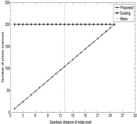
[image:6.595.319.541.354.555.2]

Now, all the pixels at the boundary will form edge pixels and remaining are inner pixels. The graph in Fig. 10 shows the plot among number of pixels processed to compute the path edge pixel versus geodesic distance.

Fig. 10: Complexity comparison of proposed algorithm with existing algorithms.

(7)

[image:7.595.59.277.72.239.2]

Fig.. 11: cumulative computation cost of algorithms for different plateau size.

It can be observed in Fig..s 10 that the number of pixels scanned by proposed algorithm is high with geodesic distance. The plateaus are always irregular in an image. For irregular

surfaces number of pixels having edge pixels at higher geodesic distance is relatively low. Therefore, the proposed algorithm performs better with natural images.

6. CONCLUSION

This paper presents an ideal approach to solve the path regularization problem existing in fast watersheds. Experimental results show that speed achieved by this method does not compromise on accuracy achieved by existing algorithms. Memory requirement of proposed algorithm is very low which makes hardware implementation feasible. Overall efficiency of proposed algorithm is above 20% when compared with fastest method proposed so far.

Table 2: Comparison of Proposed algorithm with existing algorithms.

Test Images Parameters

Existing Algorithms

Proposed Algorithm

% Improvement Vincent et. Al

[2]

Bieniek et. Al [1]

Han Sun et.al [3]

Victor et.al [9]

Lena (1024 x 1024)

Catchment Basins 19852 19852 19852 19852 19852

15.56

Running time (ms) 2565 1533 1242 951 803

Baboon (1024x1024)

14.76

Running time (ms) 2767 1509 1144 779 664

Peppers (1024x1024)

14.57

Running time (ms) 2879 1527 1220 913 780

Lena (512 x 512)

Catchment Basins ₁₀₆₅₆ ₁₀₆₅₆ ₁₀₆₅₆ ₁₀₆₅₆ ₁₀₆₅₆

22.50

Running time (ms) ₂₃₄ ₆₇ ₆₄ ₄₀ ₃₁

Baboon (512 x 512)

Catchment Basins ₁₈₁₉₇ ₁₈₁₉₇ ₁₈₁₉₇ ₁₈₁₉₇ ₁₈₁₉₇

23.24

Running time (ms) ₅₄₄ _478.72 ₂₈₇ ₁₈₅ ₁₄₂

Peppers (512 x 512)

Catchment Basins ₁₆₁₄₃ ₁₆₁₄₃ ₁₆₁₄₃ ₁₆₁₄₃ ₁₆₁₄₃

24.63

Running time (ms) 489 393 298 203 153

Brain (388 x 395)

30.70

Running time (ms) ₁₄₁ ₃₅ ₃₃ _18.76 ₁₃

Blood (272 x 265)

19.71

[image:7.595.54.546.294.589.2]

(8)

Fig.. 11. (a) Original Image (b) Result of Watershed Segmentation (c) Result of Proposed algorithm

7. REFERENCES

[1] Bieniek, A., Moga, A., An efficient watershed algorithm based on connected components. Pattern Recogn. 33 (3), pp. 907-916,2000.

[2] L. Vincent and P. Soille, ”Watershed in Digital Spaces: An Efficient Algorithm Based on Immersion Simulations,” IEEE Trans. Pattern Analysis and Machine Intelligence, vol. 13, no. 6, pp. 583-598, June 1991.

[3] Han Sun, Jingyu Yang and Mingwu Ren ”A fast watershed algorithm based on chain code and its application in image segmentation”, Pattern Recognition Letters 26, pp.1266-1274, (2005).

[4] Ramesh Jain, Rangachari Kasturi and Brian G. Schunck, ” Machine Vision”, McGraw Hill, Inc., 1995.

[5] J. Serra, Image Analysis and Mathematical Morphology. London: Academic,1982.

[6] F. Maisonneuve, ”Surle partage des eaux,” School of Mines, Paris, France, Internal Rep. CMM, 1982

[7] S. Beucher and F. Meyer, “The Morphological Approach of Segmentation: The Watershed Transformation,” Mathematical Morphology in Image Processing, E. Dougherty, ed., chapter 12, pp. 43-481, New York: Marcel Dekker, 1992

[8] A. Bleu, L.J. Leon, “Watershed-based segmentation and region merging”, Computer vision and Image Understanding, 77, (3), (2000), pp 317 – 370.

[9] Víctor Osma-Ruiz, Juan I. Godino-Llorente, Nicolás Sáenz-Lechón, Pedro Gómez-Vilda,” An improved Watershed algorithm based on efficient computation of shortest paths”, The Journal Of Pattern Recognition Society, 40, June 2006, pp1078 – 1091.

[10] R.C. Gonzalez, R.E. Woods, S.L. Eddins, “Segmentation using the watershed transform” R.C. Gonzalez, R.E. Woods, S.L. Eddins (Eds.), Digital Image Processing Using MATLAB, Pearson Prentice- Hall, NJ, USA, 2004, pp. 417–425.

[11] Bleau, J. De Guise, R. LeBlanc, “A new set of fast algorithms for mathematical morphology: I-Idempotent geodesic transforms”, CVGIP: Image Understanding 56 (2) (1992) pp.178–209.

[12] Freeman H, On The Encoding of Arbitrary Geometric ConFig.urations. IRE Trans EC-10 (2), 1961, pp.260-268

[13] F. Meyer and S. Beucher, “Morphological Segmentation,” J. Visual Comm. and Image Representation, vol. 1, no. 1, pp. 21-46, Sept. 1990.

[image:8.595.139.458.71.412.2]

(9)

[15] A.N. Moga, M. Gabbouj, Parallel image component labeling with watershed transformation, IEEE Trans. Pattern Anal. ach. Intell. 19 (5) (1997) pp.441–450.

[16] J.B.T.M. Roerdink, A. Meijster, The watershed transform: definitions, algorithms and parallelization strategies, undamenta Informaticae 41 (2000), pp.187– 228.

[17] S.Y. Chien, Y.W. Huang, S.Y. Ma, L.G. Chen, Predictive watershed for image sequences segmentation, in: Proceedings of IEEE ICASSP‟02, vol. 3, Orlando, FL, USA, May 2002, pp. 3196–3199.

[18] ZHOU Kai-jun , YANG Chun-hua , GUI Wei-hua and XU Can-hui “Clustering-driven watershed adaptive segmentation of bubble image”, J. Cent. South Univ. Technol. (2010) 17: 1049−1057 , Central South University Press and Springer-Verlag Berlin Heidelberg 2010

[19] J. Cousty, G. Bertrand, M. Couprie, L. Najman, “Fusion Graphs: Merging Properties and Watersheds”, J Math Imaging Vis (2008) 30: pp. 87–104.

[20] Erlend Hodneland , Xue-Cheng Tai, Hans-Hermann Gerdes,” Four-Color Theorem and Level Set Methods for Watershed Segmentation”, Int J Comput Vis (2009) 82: pp. 264–283.

[21] Abhinav Gupta, Bhuvan Gosain and Sunanda Kaushal, “A Comparison Of Two Algorithms For Automated Stone Detection In Clinical B-Mode Ultrasound Images Of The Abdomen”, Journal of Clinical Monitoring and Computing (2010) 24:pp. 341–362.

[22] Guifeng Zhang, Zhaocong Wu, Lina Yi, “Marker-Based Watershed Segmentation Embedded with Edge Information” 2010 IEEE

[23] Qiao Sun, Wei Yang, Lina Yu, “Research and Implementation of Watershed Segmentation Algorithm Based on CCD Infrared Images”, in First International Conference on Pervasive Computing, Signal Processing and Applications. 2010, pp.648-651.

[24] Deren Li, Guifeng Zhang, Zhaocong Wu, and Lina Yi, An Edge Embedded Marker-Based Watershed Algorithm for High Spatial Resolution Remote Sensing Image Segmentation”, IEEE Transactions On Image Processing, vol. 19, no. 10, october 2010, pp. 2781-2787.

[25] Shu Li, Lei Wu, Yang Sun, “Cell Image Segmentation Based on An Improved Watershed Transformation”, International Conference on Computational Aspects of Social Networks, 2010, pp.93-96.

[26] Lee Seng Yeong, Li-Minn Ang, Kah Phooi Seng, “3D watershed based on rainfall-simulation for volume segmentation”, in International Conference on Intelligent Human-Machine Systems and Cybernetics, 2009, pp.477-481.

[27] C. Rambabu & I. Chakrabarti, “An Efficient Hillclimbing-based Watershed Algorithm and its Prototype Hardware Architecture”, J Sign Process Syst (2008) 52:pp. 281–295.

[28] Liang Li, Yingxia Fu, Peirui Bai, Wenjie Mao, “Medical ultrasound image segmentation based on improved watershed scheme”, 2009, IEEE.