Improved Round Robin Scheduling using
Dynamic Time Quantum
Debashree Nayak
Lecturer
Gandhi Institute of Technology And
Management,Bhubaneswar, Odisha, India
Sanjeev Kumar Malla
Student
Gandhi Institute of Technology And
Management,Bhubaneswar, Odisha, India
Debashree Debadarshini
Student
Gandhi Institute of Technology And
Management,Bhubaneswar, Odisha, India
ABSTRACT
Round Robin scheduling algorithm is the widely used scheduling algorithm in multitasking and real time environment. It is the most popular algorithm due to its fairness and starvation free nature towards the processes, which is achieved by using the time quantum. As the time quantum is static, it causes less context switching incase of high time quantum and high context switching incase of less time quantum. Increasing context switch leads to high avg. waiting time, high avg. turnaround time which is a overhead and degrades the system performance. So, the performance of the system solely depends upon the choice of optimal time quantum which is dynamic in nature. In this paper, we have proposed a new variant of RR scheduling algorithm known as Improved Round Robin (IRR) Scheduling algorithm, by arranging the processes according to their shortest burst time and assigning each of them with an optimal time quantum which is able to reduce all the above said disadvantages. Experimentally we have shown that our proposed algorithm performs better than the RR algorithm, by reducing context switching, average waiting and average turnaround time.
Keywords
RR Scheduling, Context Switching, Average waiting time, Average turnaround time.
1.
INTRODUCTION
Operating System is a collection of software modules to assist programmers in enhancing system efficiency and robustness. It is an extended machine from the user’s point of view & a resource manager from the system point of view. Scheduling is the most repetitively used fundamental concept in OS. In multitasking and multiprogramming environment it is necessary to choose the process among the number of process present in the job pool according to their need. Allocation of CPU to the processes is done by scheduler, which operated by some scheduling algorithms. FCFS, SJF, Priority & RR are different type of scheduling algorithms. In which RR is the most popular non-preemptive scheduling algorithm. In non-preemption, CPU is assigned to a process until its execution is completed. But in preemption, running process is forced to release the CPU by the newly arrived process[8,9]. Each scheduling algorithm has its own advantages and disadvantages. Similarly RR has a drawback which increase average waiting time, average turnaround time and minimizes the throughput, known as Context switch. The processes in RR are assigned with a time quantum which is static by nature.
1.1
Preliminaries
A program in execution is called a process. The processes waiting to be assigned to a processor are put in a queue called ready queue. The time for which a process holds the CPU is known as burst time. Arrival Time is the time at which a process arrives at the ready queue. Turnaround time is the total time taken by a process from its submission to its completion. Waiting time is the amount of time a process has been waiting in the ready queue. The number of times CPU switches from one process to another is known as context switch.
1.2
Scheduling Algorithms
In the First-Come-First-Serve (FCFS) algorithm, the CPU is assigned immediately to that process which arrives first at the ready queue. In Shortest Job First (SJF) algorithm, process having shortest CPU burst time will execute first. If two processes having same burst time and arrival time, then FCFS procedure is followed. Priority scheduling algorithm, provides the priority to each process and selects the highest priority process from the ready queue. A small unit of time quantum is given to each process present in the ready queue in case of Round Robin (RR)algorithm which maintains the fairness factor.
1.3
Motivation
In RR scheduling, processes get fair share of CPU because of static time quantum assign to each process and the context switch is inversely proposnal to choice of static time quantum which degrades the overall performance of the system (high average waiting time & average turnaround time). This factor motivates us to design an improved algorithm which is able to increase the system performance by reducing the number of context switches, average waiting time & average turnaround time using the concept of dynamic time quantum.
1.4
Related Work
The static time quantum which is a limitation of RR was removed by taking dynamic time quantum using median method introduced in SARR algorithm[2]. In DQRRR [1] the median method and job mix concept is reused in a different way. DQRRR gives better result than the classical RR scheduling algorithm. Recently a number of new variants of Improved RR algorithms have been developed in [3-7].
1.5
Our Contribution
1.6
Organization of Paper
Section 2 presents the proposed approach. Section 3 shows experimental analysis. The whole work is concluded and the future scope is discussed in section 4.
2.
PROPOSED APPROACH
In our proposed algorithm, we are arranging the processes in ascending order according to their burst time present in the ready queue. For finding an optimal time quantum, median method is followed. The median can be calculated using the following formulae[2].
Median (M) =
Y
Y
ifniseven
ifnisodd
Y
n n n 2 1 2 2 22
1
Where, M = median
Y = number located in the middle of a group of numbers arranged in ascending order
n = number of processes
Then, the optimal time quantum is calculated as follows : Optimal Time Quantum (Oqt) =
2
) (M Median
HighestBt
The optimal time quantum is assigned to each processes and is recalculated taking the remaining burst time in account after each cycle. This procedure goes on until the ready queue is empty.
2.1
Proposed Algorithm
1. I/P: Process(Pn), Burst Time(bt), Arrival Time, ready queue. O/P: Context Switch(Cs), Avg.WaitingTime(Awt), Avg.Turnarround Time(Att)
2. Initialize: ready queue=0, Cs=0, Awt=0, Att=0 3. While (ready queue!=0)
// Sort the processes in ascending order according to their Bt in ready queue
//Find Median //Calculate Oqt
1. //assign Oqt to each process For each process i=1 to n P[i] Oqt
2. If new process arrives Update counter and goto step3 end while
3. Cs, Awt, Att are calculated. 4. Stop and exit.
2.2
Illustration
To demonstrate the above algorithm we have considered the following example. Arrival time is considered to be zero for the given processes P1, P2, P3, P4 and corresponding burst times are 60, 20, 80, 40 respectively. In first step the processes in the ready queue are sorted in ascending order. Then the time quantum is calculated in the second step. Here
P1 with bt=60 and P3 with bt=80. After assigning Oqt to each process the remaining burst time of all process are P1=0, P2=0, P3=15 and P4=0. When a process completes its execution, it is deleted from ready queue automatically. Then the next time quantum is calculated from remaining burst times as per the 3rd step in the algorithm. Here Oqt=15. Then the remaining burst times are P3=0.In the last step P3 will complete its execution and will be deleted from the ready queue.
3.
EXPERIMENTAL ANALYSIS
3.1
Assumptions
All the processes are assumed to be independent. Time slice is assumed to be not more than the maximum burst time. All the attributes like burst time, number of processes and the time slice of all the processes are known before submitting the processes to the processor. All processes are CPU bound. No processes are I/O bound.
3.2
Experimental Frame Work
Our experiment consists of several input and output parameters. The input parameters consist of burst time(Bt), arrival time(At), optimal time quantum(Oqt) and the number of processes(Pn). The output parameters consist of average waiting time(Awt), average turnaround time(Att) and number of context switches(Cs).
3.3
Result Obtained
Our proposed algorithm can work effectively with large number of data. In each case we have compared our proposed algorithm’s results with Round Robin scheduling algorithm’s result. For RR Scheduling Algorithm we have taken 25 as the static time quantum.
Case 1: With Zero Arrival Time
Increasing Order
We consider five processes P1, P2, P3, P4 and P5 arriving at time 0 with burst time 30, 34, 62, 74, 88 respectively shown in Table 3.1. Table 3.2 shows the comparing result of RR algorithm and our proposed algorithm.
Table 1. Data in Increasing Order
Table 2. Comparison between RR and IRR
No. of process At Bt
P1 0 30
P2 0 34
P3 0 62
P4 0 74
P5 0 88
Algorithm RR IRR
qt 25 75,13
Cs 13 5
Awt 149 85.6
Fig 1: Gantt chart for RR in Table 2
Fig 2: Gantt chart for IRR in Table 2
Decreasing Order
We consider five processes P1, P2, P3, P4 and P5 arriving at time 0 with burst time 77, 54, 45, 19, 14 respectively shown in Table 3. Table 4 shows the comparing result of RR algorithm and our proposed algorithm.
Table 3. Data in Decreasing Order
Table 4. Comparison between RR and IRR
Fig 3: Gantt chart for RR in Table 4
Fig 4: Gantt chart for IRR in Table 4
Random Order
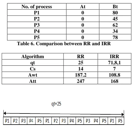
We consider five processes P1, P2, P3, P4 and P5 arriving at time 0 with burst time 80, 45,62,34,78 respectively shown in Table 3.5.Table 3.6 shows the comparing result of RR algorithm and our proposed algorithm.
Table 5. Data in Random Order
[image:3.595.90.233.155.211.2]Table 6. Comparison between RR and IRR
Fig 5: Gantt chart for RR in Table 6
Fig 6: Gantt chart for IRR in Table 6
Case 2: Without Zero Arrival Time
Increasing Order
We consider five processes P1, P2, P3, P4 and P5 arriving at time 0,2,6,8,14 and burst time 14,34,45,62,77 respectively shown in Table 3.7. Table 3.8 shows the comparing result of RR algorithm and our proposed algorithm.
Table 7. Data in Increasing Order
Table 8. Comparison between RR and IRR
No. of process At Bt
P1 0 77
P2 0 54
P3 0 45
P4 0 19
P5 0 14
Algorithm RR IRR
qt 25 61,16
Cs 10 5
Awt 117.4 51.4
Att 159.2 93.2
No. of process At Bt
P1 0 14
P2 2 34
P3 6 45
P4 8 62
P5 14 77
No. of process At Bt
P1 0 80
P2 0 45
P3 0 62
P4 0 34
P5 0 78
Algorithm RR IRR
qt 25 71,8,1
Cs 14 7
Awt 187.2 108.8
Att 247 168
Algorithm RR IRR
qt 25 14,65,12
Cs 11 5
Awt 97 56.6
[image:3.595.50.280.345.414.2] [image:3.595.316.551.588.734.2]Fig 7: Gantt chart for RR in Table 8
Fig 8: Gantt chart for IRR in Table 8
Decreasing Order
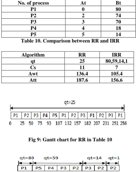
We consider five processes P1, P2, P3, P4, P5 arriving at time 0,2,3,4,5 and burst time 80,74,70,18,14 respectively shown in Table 3.9. Table 3.10 shows the comparing result of RR algorithm and our proposed algorithm.
Table 9. Data in Decreasing Order
[image:4.595.318.550.97.596.2]Table 10. Comparison between RR and IRR
Fig 9: Gantt chart for RR in Table 10
Fig 10: Gantt chart for RR in Table 10
Random Order
We consider five processes P1, P2, P3, P4 & P5 arriving at time 0, 1,4,6,7 and burst time 65,72,50,43,80 respectively
Table 11. Data in Random Order
Table 12. Comparison between RR and IRR
Fig 11: Gantt chart for RR in Table 12
Fig 12: Gantt chart for IRR in Table 12
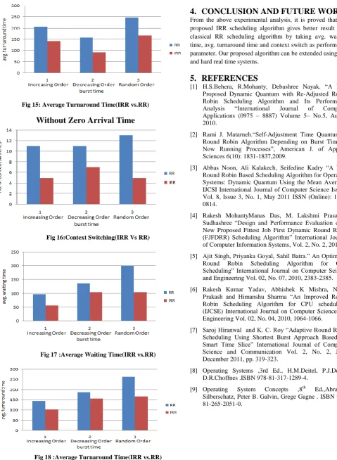
With Zero Arrival Time
Fig 13: Context Switching(IRR vs. RR)
Fig 14 :Average Waiting Time(IRR vs.RR)
No. of process At Bt
P1 0 80
P2 2 74
P3 3 70
P4 4 18
P5 5 14
Algorithm RR IRR
qt 25 80,59,14,1
Cs 11 7
Awt 136.4 105.4
Att 187.6 156.6
No. of process At Bt
P1 0 65
P2 1 72
P3 4 50
P4 6 43
P5 7 80
Algorithm RR IRR
qt 25 72,8
Cs 13 5
Awt 199.8 104.8
[image:4.595.90.244.171.227.2] [image:4.595.46.280.361.657.2]Fig 15: Average Turnaround Time(IRR vs.RR)
Without Zero Arrival Time
Fig 16:Context Switching(IRR Vs RR)
[image:5.595.45.525.63.718.2]Fig 17 :Average Waiting Time(IRR vs.RR)
Fig 18 :Average Turnaround Time(IRR vs.RR)
4.
CONCLUSION AND FUTURE WORK
From the above experimental analysis, it is proved that our proposed IRR scheduling algorithm gives better result than classical RR scheduling algorithm by taking avg. waiting time, avg. turnaround time and context switch as performance parameter. Our proposed algorithm can be extended using soft and hard real time systems.
5.
REFERENCES
[1] H.S.Behera, R.Mohanty, Debashree Nayak. “A New Proposed Dynamic Quantum with Re-Adjusted Round Robin Scheduling Algorithm and Its Performance Analysis “International Journal of Computer Applications (0975 – 8887) Volume 5– No.5, August 2010.
[2] Rami J. Matarneh.“Self-Adjustment Time Quantum in Round Robin Algorithm Depending on Burst Time of Now Running Processes”, American J. of Applied Sciences 6(10): 1831-1837,2009.
[3] Abbas Noon, Ali Kalakech, Seifedine Kadry “A New Round Robin Based Scheduling Algorithm for Operating Systems: Dynamic Quantum Using the Mean Average” IJCSI International Journal of Computer Science Issues, Vol. 8, Issue 3, No. 1, May 2011 ISSN (Online): 1694-0814.
[4] Rakesh MohantyManas Das, M. Lakshmi Prasanna, Sudhashree “Design and Performance Evaluation of A New Proposed Fittest Job First Dynamic Round Robin (FJFDRR) Scheduling Algorithm” International Journal of Computer Information Systems, Vol. 2, No. 2, 2011. [5] Ajit Singh, Priyanka Goyal, Sahil Batra.” An Optimized
Round Robin Scheduling Algorithm for CPU Scheduling” International Journal on Computer Science and Engineering Vol. 02, No. 07, 2010, 2383-2385. [6] Rakesh Kumar Yadav, Abhishek K Mishra, Navin
Prakash and Himanshu Sharma “An Improved Round Robin Scheduling Algorithm for CPU scheduling” (IJCSE) International Journal on Computer Science and Engineering Vol. 02, No. 04, 2010, 1064-1066.
[7] Saroj Hiranwal and K. C. Roy “Adaptive Round Robin Scheduling Using Shortest Burst Approach Based On Smart Time Slice” International Journal of Computer Science and Communication Vol. 2, No. 2, July-December 2011, pp. 319-323.
[8] Operating Systems ,3rd Ed., H.M.Deitel, P.J.Deitel, D.R.Choffnes .ISBN 978-81-317-1289-4.