Measuring trade efficiency

Munich Personal RePEc Archive

Measuring trade efficiency

Halkos, George and Tzeremes, Nickolaos

University of Thessaly, Department of Economics

13 September 2005

Online at

https://mpra.ub.uni-muenchen.de/23761/

Discussion Paper 05/05, University of Thessaly,

Department of Economics

Measuring trade efficiency

by

George Emm. Halkos

and Nickolaos

G.

Tzeremes

Department of Economics, University of Thessaly Argonavton and Filellinon st., 38221, Volos, Greece

Abstract

In this paper we use the Data Envelopment Analysis (DEA) window method to compare trade efficiency for 16 OECD countries and for the time period 1996– 2000. From the analysis we obtained the efficiency scores and the optimal output levels for inefficient countries for all years under consideration. Results drawn from the broadly used ratio analysis were also compared to those derived from the DEA model. It seems that trade efficient countries have clear characteristics. These are the low exchange rates for exports, low R&D intensity, high value intra industry trade, and with positive effect of trade on their GDP.

JEL Classification: F1, O1

I. Introduction

In this paper we use Data Envelopment Analysis (hereafter DEA) window method to

compare trade efficiency for 16 OECD countries and for the time period 1996–2000. For this

reason we use for the first time in this type of formulation a number of ratios. Namely, we use

and construct indicators for the Research and Development intensity of each country in terms

of production, the value added shares from the manufacturing sector relative to the total

economy, the intra industry trade, the net trade to GDP and the exchange rates. From the

analysis we obtained the efficiency scores and the optimal output (ratios) levels for inefficient

countries for all the five years under consideration. Results drawn from the broadly used ratio

analysis were also compared to the results derived from the DEA window model.

The paper is organized as follows. In section II the technique adopted both in its

theoretical and mathematical formulation is presented. Section III discusses the ratios used in

the formulation of the proposed model. In section IV the empirical findings of our study are

presented. The final section concludes the paper discussing the derived results and the implied

policy implications.

II. The proposed model

Consider N DMUs (in our case 16 OECD countries), each producing m products using

n inputs. Efficiency is measured as:

1 1

/

m n

k ik ik jk jk

i j

f b y c x

= =

=

∑

∑

Where yik (>0) is the amount of output i by the kth DMU, xjk (>0 ) is the amount of input j

used by the kth DMUs, bik and cjk are the output and the input respectively. The efficiency

1 1

/

1

m n

ik ik jk jk

i j

b y

c x

= =

≤

∑

∑

and bi k , c j k ≥ 0 (3)

According to the first inequality the efficiency ratios cannot exceed one, while

according to the second the weights are positive and are determined by DEA in such a way as

each DMU maximises its own efficiency ratio.

The problem can be formulated as an ordinary linear program. That is:

Maximize

1

1

m

k ik ik

i ik il i

f

b

y

c x

⎛

⎞

⎜

⎟

=

_⎜

_⎟

⎜

⎟

⎝

⎠

∑ ∑

subject to

1 1

1

1

0

m n

ik ik jk jl

i ik il j jk jl

i j

b

y

c

x

c x

c x

= =

⎛

⎞

⎛

⎞

⎜

⎟

⎜

⎟

₋

_≤

⎜

⎟

⎜

⎟

⎜

⎟

⎜

⎟

⎝

⎠

_⎝

_⎠

∑

_∑

∑

_∑

1

1

1

n

i k j k

j j k j l

j b x c x = ⎛ ⎞ ⎜ ⎟ ₌ ⎜ ⎟ ⎜ ⎟ ⎝ ⎠

∑ ∑

and 1 ik 0, 1 jk 0

ik il jk jl

i j

b c

c x c x

⎛ ⎞ ⎛ ⎞ ⎜ ⎟ ⎜ _{⎟ ≥ ≥} ⎜ ⎟ ⎜ ⎟ ⎜ ⎟ ⎜ ⎟ ⎝

∑

∑

The corresponding dual problem can be expressed as:

Minimize

1 1

m n

k lk jk

i j

s

s

θ τ

= =

⎛

⎞

−

_⎜

+

_⎟

⎝

∑

∑

⎠

subject to

0

N

kl il il lk

l

y

y

s

λ

₋

₋

₌

∑

i

=

1, ...

m

0

N

k

x

x

s

θ

₋

∑

λ

₋

₌

,

,

0

kl

s

s

λ

_≥

(11)

By linear programming duality theory, the optimal value of θk (the overall technical

efficiency) equals the optimal value of fk (θk lies between zero and one). In (8), τ represents

an arbitrarily small positive number and ensures that the optimal solutions are at finite

non-zero external points and that the optimal solutions are at finite non – non-zero extremal points. It

also ensures that the slack in input j does not affect the optimal value of fk.

Technical efficiency is achieved only when θk=1 (ensuring that DMUs is on the

frontier) and Slk+ = Sjk- = 0 (excluding external points). An inefficient DMU can become

efficient by adjusting output and inputs as follows:

*

lk lk lk

y

=

y

+

s

and

*

jk k jk jk

x

=

θ

x

−

s

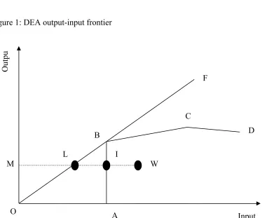
Figure 1: DEA output-input frontier

F

D C

W I

A L

B

M

Input

Outpu

The problem in (8) through (11) assumes constant returns to scale (CRS). Figure 1 illustrates

the approach using one output and one input. The frontier OF is the solution of the formulated

problem in (8)-(11). Countries on the frontier have an efficiency score of one. Countries

located inside the frontier have an efficiency score of less than one. For example, country s

located at point W is inefficient, and the overall technical efficiency is measured by the ratio

ML/MW.

The overall technical efficiency can be broken into pure technical and scale efficiency.

To do that we solve the above linear programming problem with the additional restriction that

1

N lk l

λ

=

∑

which allows for variable returns to scale (VRS). In figure 1, the VRS case is represented by

the ABCD frontier. The pure technical efficiency of country s located at point W is given by

the ratio MI/MW= κs. The degree of scale efficiency is computed as

ζ

=

θ κ

/

construction κs exceeds θs. If the value of ζs is one the country is scale efficient. If scale

inefficiency exists, it can be due to either increasing or decreasing returns to scale (IRS or

DRS). To differentiate IRS from DRS, we solve again the same linear programming problem

with the additional restriction of

1

N lk l

λ

≤

∑

which allows for non-increasing returns to scale (NIRS). In figure 1, this case is represented

by the OBCD frontier. For country s located at point W, the efficiency is given by

/

s ML MW

φ = , which also equals θs. By construction, φs≥θs and φs≤ κs, if φs= κs and scale

inefficiency exists, then it is due to decreasing returns to scale. If κs≠φs, then the scale

The DEA model illustrated above has been introduced by Charnes et al. (1978);

however a variation of this model will be used based on moving averages introduced by

Charnes et al. (1985). The use of this variation is due to its ability to handle multiple outputs

and inputs and their efficiencies over time (Charnes et al. 1994). Asmid et al. (2004),

highlight the fact that there are no technical changes within each of the windows because all

DMUs in each window are measured (compared) against each other and suggest that in order

for the results to be credible a narrow window width must be used. Adopting the

formalization by Asmild et al. (2004) consider the N DMU’s (n=1,…N) observed for T

periods (t=1,..T) using r inputs and s outputs. So this will create a sample of N x T

observations where an observation n in period t, (DMU_tn) has an r dimensional input vector

(

)

n n n n

t t t rt

x = x x x ′and an s dimensional output vector y_tn =

(

)

Then a window kw with k x w observations is denoted starting at time k, 1≤ ≤k T with

width w, 1≤ ≤ −w T k. So the matrix of inputs is given as:

(

)

1 1 1

, ,...., N, , ,...., N , , ,...., N

kw k k k k k k k w k w k w

X = x x x x ₊ x ₊ x ₊ x ₊ x ₊ x ₊

and the matrix of outputs will be:

(

)

1 1 1

, ,...., N, , ,...., N , , ,...., N

kw k k k k k k k w k w k w

y = y y y y ₊ y ₊ y ₊ y ₊ y ₊ y ₊

The output oriented DEA window problem for DMU_t' under the CRS assumption is given by

solving the linear program illustrated below:

,

' '

max

. .

0

0

0, (

1,...,

)

kw t

kw t

n

s t

X

x

Y

y

n

N w

θ λ

θ

λ θ

λ

λ

−

−

+

≥

−

≥

≥

=

∗

III. Data

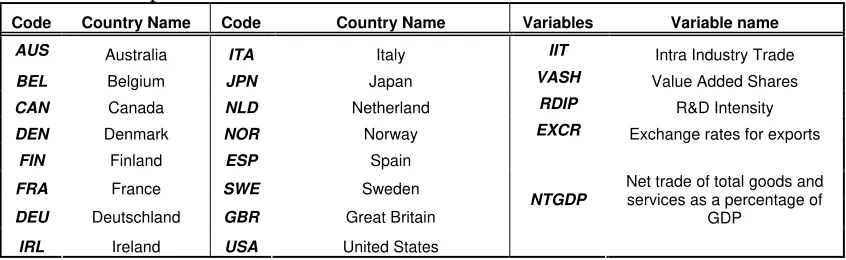
Using data for 16 OECD countries (Table 1) from “Bilateral Trade Database”1 and for

a time span of five years (1996-2000) a number of ratios were constructed and are used in our

empirical analysis.

Table 1: Description and variable codes.

Code Country Name Code Country Name Variables Variable name

AUS _{Australia ITA Italy} IIT _{Intra Industry Trade}

BEL Belgium JPN Japan VASH Value Added Shares

CAN Canada NLD Netherland RDIP R&D Intensity

DEN Denmark NOR Norway EXCR Exchange rates for exports

FIN Finland ESP Spain

FRA France SWE Sweden

DEU Deutschland GBR Great Britain

IRL Ireland USA United States

NTGDP

Net trade of total goods and services as a percentage of

GDP

Specifically, the first ratio is an indicator showing the R&D intensity of each country

in terms of production (RDIP). That is:

100

k k

k

ANBERD

RDIP

PROD

=

∗

Where ANBERD _and PROD _{are business enterprise Research and Development and}

production at current prices respectively. For each country this indicator expresses the R&D

expenditures by the total manufacturing sector relative to the production.

This ratio was constructed in order to approach the concern of a country to deal with

technological developments and the speed with which the country adapts them.

The second ratio shows the value added shares from manufacturing sector relative to

the total economy (VASH). That is

100

K i

i K

total

VALU

VASH

VALU

⎡

⎤

=

_⎢

_⎥

∗

⎣

⎦

Where VALU is the value added at current prices. For a given country, this indicator shows

industries. The valuation of value added differs among countries and may therefore influence

the interpretation of this indicator. Value added is measured at basic prices for all countries

except JAPAN and the USA, which are used in producer or market prices.

The third indicator shows the intra industry trade (IIT). This aspect of the structure of

international trade has not received much attention in the existing trade performance

literature. In our construction it is expressed as:

(

)

(

)

. .

1

100

k k

i i

k i

tot manuf _{k k}

i i i

EXPO

IMPO

IIT

EXPO

IMPO

⎡

₋

⎤

⎢

⎥

= −

_⎢

_⎥

∗

+

⎢

⎥

⎣

⎦

∑

∑

where EXPO and IMPO are the total exports and imports of goods at current prices. Intra

industry trade is the value of total trade remaining after subtraction of the absolute value of

net exports and imports of manufacturing industry. For comparison, between countries this

measure is expressed as a percentage of manufacturing industry’s combined exports and

imports. This index ranges from 0 to 100. If a country exports and imports roughly equal

quantities of certain products, the IIT index is high. If trade is mainly one-way (whether

exporting or importing), the IIT index is low.

Figure 2: (a) Exchange rate for exports; (b) Value added shares; (c) Intra-Industry Trade; (d) R&D Intensity; (e) NTGDP; (f) GDP.

(1a) 0,000000 0,100000 0,200000 0,300000 0,400000 0,500000 0,600000 0,700000 0,800000 0,900000 1,000000 1,100000 1,200000 1,300000 1,400000 1,500000 1,600000 1,700000 1,800000

AUS BEL CAN DEN FIN FRA DEU IRL ITA JPN NLD NOR ESP SWE GBR USA

Countries e x c h a n g e r a te fo r e x p o rts d o lla rs p e r lo c a l c u rr e n c y 1996 1997 1998 1999 2000 (1b) 0,00 1,50 3,00 4,50 6,00 7,50 9,00 10,50 12,00 13,50 15,00 16,50 18,00 19,50 21,00 22,50 24,00 25,50 27,00 28,50 30,00 31,50 33,00 34,50

AUS BEL CAN DEN FIN FRA DEU IRL ITAJPN NLD NOR ESP SWE GBR USA

(1c) 0,00 4,00 8,00 12,00 16,00 20,00 24,00 28,00 32,00 36,00 40,00 44,00 48,00 52,00 56,00 60,00 64,00 68,00 72,00 76,00 80,00 84,00 88,00 92,00 96,00

AUS BEL CAN DEN FIN FRA DEU IRL ITAJPN NLD NOR ESP SWE GBR USA

Countries in tr a in d u s tr y t ra d e 1996 1997 1998 1999 2000 (1d) 0,00 0,20 0,40 0,60 0,80 1,00 1,20 1,40 1,60 1,80 2,00 2,20 2,40 2,60 2,80 3,00 3,20 3,40 3,60 3,80 4,00 4,20

AUS BEL CAN DEN FIN FRA DEU IRL ITAJPN NLD NOR ESP SWE GBR USA

Countries R & D In te n s it y ₁₉₉₆ 1997 1998 1999 2000 (1e) -2,5-2 -1,5-1 -0,50 0,51 1,52 2,53 3,5 4 4,55 5,56 6,57 7,58 8,59 9,510

AUS BEL CAN DEN FIN FRA DEU IRL ITA JPN NLD NOR ESP SWE GBR USA

Countries N e t t ra de of t ot a l g oods a nd s e rv ic e s as a % o f G D P 1996 1997 1998 1999 2000 (1f) 0 1000000 2000000 3000000 4000000 5000000 6000000 7000000 8000000 9000000 10000000

AUS BEL CAN DEN FIN FRA DEU IRL ITA JPN NLD NOR ESP SWE GBR USA Countries GD P 1996 1997 1998 1999 2000

Furthermore, the ratio NTGDP has been constructed in order to indicate the

contribution of net trade to GDP of each country. That is:

NTGDP = [(Exports of commodities – Imports of commodities)/ GDP] * 100 (20)

Finally, an indicator of the exchange rate for exports for each country (dollars per local

currency) EXCR has been used.

IV. Empirical Results

Using a conventional ratio analysis as presented graphically in Figure 1a-f

different conclusions can be derived looking at the countries from six different measurement

perspectives. For instance looking at the performance of the exchange rate for exports and in

the case of Great Britain (Figure 1a) an increase over the five years can be observed.

Furthermore, the prices of the exchange rate for exports for Great Britain are significantly

higher compared to other countries. The main reason behind this may be attributed to the fact

that Great Britain has a “strong” currency.

Significantly different is the performance of the EXCR of Ireland compared to other

value added contributed by manufacturing sector relative to total value added for all its

industries, while Norway has the lowest compared to the other countries.

Figure 1c, illustrates the intra industry trade of manufacturing for each country over

the years. Australia and Japan have the lowest performance in terms of exports and imports at

current prices. The highest price is observed for Belgium, France, Great Britain, the

Netherlands and Spain. Moderate, trade performance has been noticed for the USA, Canada,

Denmark and Sweden.

Looking at figure 1d the performance of countries in terms of their R&D expenditure

over the five years time period can be observed. We notice that Sweden, Japan and the USA

have a significant higher performance in terms of R&D expenditure compared to the other

countries. A medium performance is highlighted for Germany, France, Finland and Great

Britain. The lowest performance has been noticed for Spain and Italy. Figure 1e indicates the

net trade of commodities as a percentage of GDP. Observing the performance of countries we

realize that Finland, Norway, Sweden and the Netherlands have the highest contribution to

their GDP from trade, whereas Australia, Great Britain and the USA have a negative

contribution. In the case of Norway the first 4 years present a tremendous increase of trade as

its economy was based mainly on exports, while an even greater reduction for net trade

performance for the last year under consideration can be noticed.

Finally, all the above conventional analysis must be viewed and compared along with

the last graph illustrated in figure 1f in order to have a clear view of trade efficiency and its

impact on economic development for the countries examined. That is, Figure 1f illustrates

GDP at current prices over the years.

Using conventional ratio analysis shows us the performance of the countries under

review but from (in our case) six different angles. However, it is difficult to have a clear view

insights of the factors that affect trade efficiency. In order to overcome the problem of

“multiple views” we use DEA modeling to observe trade efficiency in terms of a number of

inputs and outputs, which will provide us with a unified and simultaneous picture of trade

efficiency among the countries considered.

To perform an analysis focusing interest on changes in efficiency over time DEA

window analysis may be used. In such a case moving average analogue can be applied in

order to perform DEA overtime. DMUs in each period are treated as if they were different

DMU. A DMU’s performance in a particular period is contrasted with its performance in

other periods in addition to the performance of the other DMUs.

In our case the DMUs are the OECD countries (n=16) over five years period (p=5)

and we proceed our analysis by using a three –year (w=3) window. Each DMU (country) is

represented as if it was a different DMU for each of the three years in the first window (Years

1, 2 and 3). An analysis of the 48 (nw = 3 x 16) DMUs is taking place. The window is then

moved one period by replacing Year 1 with Year 4, and an analysis is performed on the

second three year set (Years 2, 3 and 4) of these 48 DMUs. The process continues moving the

window one period and concluding with the final (third) analysis of 48 DMUs for the last

three years (Years 3, 4 and 5). This procedure implies p-w+1 separate analyses, where each

analysis examines n*w DMUs.

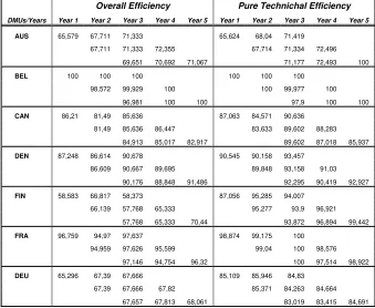
Table 2a illustrates the results of the analysis in the form of overall efficiency and pure

technical efficiency while Table 2b presents the scale efficiency scores for the performance of

the 16 OECD countries considering the VASH, RDIP and EXCR as inputs and the IIT and

NTGDP ratios as outputs. The underlying framework of the window analysis is illustrated on

this table. For the first window, Australia (AUS) is represented in the constrains of the DEA

model as if it was a different DMU in years 1, 2 and 3. Therefore, when Australia is evaluated

constraint sets along with similar performance data of the other OECD countries for Years 1,

2 and 3. Concluding, the results of the first window analysis include all the 48 efficiency

scores under the column headings for Years 1 to 3 in the first row of each OECD country.

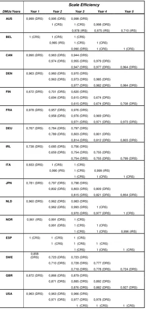
Scale efficiency scores are calculated by dividing overall efficiency by pure efficiency

as can be found in Coelli et al. (2001). If the overall efficiency and pure technical efficiency

of a DMU (country) are equal then the scale efficiency is 1. If, however, the DMU has lower

overall efficiency compared to pure technical efficiency its scale efficiency will be below 1

(Thanassoulis, 2001). A lower overall efficiency score compared to pure technical efficiency

score suggests that a country is efficient in trade terms in the former case and less efficient

when we control for scale size (in trade terms). This means that scale operation does impact

the trade efficiency of the country. Therefore, the larger the divergence between overall and

pure technical efficiency scores the lower the value of scale efficiency (in trade terms) and the

more adverse the impact of scale size on trade efficiency. Scale scores results are presented in

Table 2 (a): Window Analysis; Overall Efficiency, Pure Technical Efficiency.

Overall Efficiency Pure Technichal Efficiency

DMUs/Years Year 1 Year 2 Year 3 Year 4 Year 5 Year 1 Year 2 Year 3 Year 4 Year 5 AUS 65,579 67,711 71,333 65,624 68,04 71,419

67,711 71,333 72,355 67,714 71,334 72,496

69,651 70,692 71,067 71,177 72,493 100

BEL 100 100 100 100 100 100

98,572 99,929 100 100 99,977 100

96,981 100 100 97,9 100 100

CAN 86,21 81,49 85,636 87,063 84,571 90,636

81,49 85,636 86,447 83,633 89,602 88,283

84,913 85,017 82,917 89,602 87,018 85,937

DEN 87,248 86,614 90,678 90,545 90,158 93,457

86,609 90,667 89,695 89,848 93,158 91,03

90,176 88,848 91,486 92,295 90,419 92,927

FIN 58,583 66,817 58,373 87,056 95,285 94,007

66,139 57,768 65,333 95,277 93,9 96,921

57,768 65,333 70,44 93,872 96,894 99,442

FRA 96,759 94,97 97,637 98,874 99,175 100

94,959 97,626 95,599 99,04 100 98,576

97,146 94,754 96,32 100 97,514 98,922

IRL 58,723 53,521 64,938 79,51 78,108 85,895

51,242 64,144 62,625 77,677 84,975 82,89

64,144 62,593 63,288 84,975 82,89 79,192

ITA 84,819 100 100 90,816 100 100

99,061 100 95,867 100 100 95,924

100 95,855 100 100 95,865 100

JPN 33,422 38,176 41,741 42,741 47,876 52,267

38,176 41,741 42,038 47,556 51,918 51,948

41,736 42,033 43,508 51,151 51,182 50,889

NLD 96,065 96,27 98,307 100 100 100

96,27 98,307 99,984 100 98,923 100

95,96 97,7 100 98,829 100 100

NOR 96,121 91,231 100 100 92,027 100

91,231 100 100 91,97 100 100

100 100 93,24 100 100 93,565

ESP 100 100 100 100 100 100

100 100 100 100 100 100

100 100 100 100 100 100

SWE 72,94 69,763 69,107 84,995 96,422 95,565

68,074 69,082 77,055 95,745 94,892 99,145

68,035 77,055 68,452 94,752 99,014 94,508

GBR 83,228 83,688 85,226 95,442 96,624 96,865

83,688 85,226 85,586 95,978 96,217 95,92

83,136 83,404 87,425 94,797 94,504 94,267

USA 85,457 86,658 90,121 88,684 89,968 93,269

86,658 90,121 92,038 89,202 92,161 94,031

Table 2 (b): Window Analysis; Scale Efficiency.

Scale Efficiency

DMUs/Years Year 1 Year 2 Year 3 Year 4 Year 5 AUS 0,999 (DRS) 0,995 (DRS) 0,998 (DRS)

1 (CRS) 1 (CRS) 0,998 (DRS)

0,978 (IRS) 0,975 (IRS) 0,710 (IRS)

BEL 1 (CRS) 1 (CRS) 1 (CRS)

0,985 (IRS) 1 (CRS) 1 (CRS)

0,990 (DRS) 1 (CRS) 1 (CRS)

CAN 0,990 (DRS) 0,963 (DRS) 0,944 (DRS)

0,974 (DRS) 0,955 (DRS) 0,979 (DRS)

0,947 (DRS) 0,977 (DRS) 0,964 (DRS)

DEN 0,963 (DRS) 0,960 (DRS) 0,970 (DRS)

0,963 (DRS) 0,973 (DRS) 0,985 (DRS)

0,977 (DRS) 0,982 (DRS) 0,984 (DRS)

FIN 0,672 (DRS) 0,701 (DRS) 0,620 (DRS)

0,694 (DRS) 0,615 (DRS) 0,674 (DRS)

0,615 (DRS) 0,674 (DRS) 0,708 (DRS)

FRA 0,978 (DRS) 0,957 (DRS) 0,976 (DRS)

0,958 (DRS) 0,976 (DRS) 0,969 (DRS)

0,971 (DRS) 0,971 (DRS) 0,973 (DRS)

DEU 0,767 (DRS) 0,784 (DRS) 0,797 (DRS)

0,789 (DRS) 0,803 (DRS) 0,801 (DRS)

0,814 (DRS) 0,812 (DRS) 0,803 (DRS)

IRL 0,738 (DRS) 0,685 (DRS) 0,756 (DRS)

0,659 (DRS) 0,754 (DRS) 0,755 (DRS)

0,754 (DRS) 0,755 (DRS) 0,799 (DRS)

ITA 0,933 (DRS) 1 (CRS) 1 (CRS)

0,990 (IRS) 1 (CRS) 0,999 (IRS)

1 (CRS) 1 (CRS) 1 (CRS)

JPN 0,781 (DRS) 0,797 (DRS) 0,798 (DRS)

0,802 (DRS) 0,803 (DRS) 0,809 (DRS)

0,815 (DRS) 0,821 (DRS) 0,854 (DRS)

NLD 0,960 (DRS) 0,962 (DRS) 0,983 (DRS)

0,962 (DRS) 0,993 (DRS) 1 (CRS)

0,970 (DRS) 0,977 (DRS) 1 (CRS)

NOR 0,961 (IRS) 0,991 (DRS) 1 (CRS)

0,991 (DRS) 1 (CRS) 1 (CRS)

1 (CRS) 1 (CRS) 0,996 (IRS)

ESP 1 (CRS) 1 (CRS) 1 (CRS)

1 (CRS) 1 (CRS) 1 (CRS)

1 (CRS) 1 (CRS) 1 (CRS)

SWE

0,858

(DRS) 0,723 (DRS) 0,723 (DRS)

0,710 (DRS) 0,728 (DRS) 0,777 (DRS)

0,718 (DRS) 0,778 (DRS) 0,724 (DRS)

GBR 0,872 (DRS) 0,866 (DRS) 0,879 (DRS)

0,871 (DRS) 0,885 (DRS) 0,892 (DRS)

0,876 (DRS) 0,882 (DRS) 0,927 (DRS)

USA 0,963 (DRS) 0,963 (DRS) 0,966 (DRS)

0,971 (DRS) 0,977 (DRS) 0,978 (DRS)

Table 2b. As it can be observed, for instance Canada has a low pure technical

efficiency score in year 5 of 0.8594 or 85.94% and relatively high scale efficiency (0.964).

This means that the overall trade inefficiency of that country in the overall efficiency model

(0.8292 or 82.92%) is attributed mainly to inefficient trade policies and comparative

disadvantages. The same holds also for other countries such as Denmark, Japan and Norway.

On the other hand, if a country has an optimal pure technical efficiency score (100)

and low scale efficiency score this may imply that the trade overall inefficiency is attributed

to comparative disadvantages conditions. Australia may be viewed as an example of this case,

where it has an optimal pure technical efficiency (year 5) and a relative scale efficiency score

of 0.71. Finally, our results show that Australia and Norway display increasing returns to

scale, while Belgium, Italy, the Netherlands, and Spain exhibit constant returns to scale and

the rest of the countries decreasing returns to scale.

Table 3 decomposes overall average efficiency scores for each country in each

window, clarifying trends of trade efficiencies over the years. Moreover, in the same lines,

pure technical efficiency has been decomposed. Countries can be distinguished into three

different groups. Namely, countries with an overall efficiency over 90% (Group 1), with an

overall efficiency between 80% and 90% (Group 2) and with overall trade efficiency below

80% (Group 3). The first group includes Belgium, France, Italy, Netherlands, Norway, and

Spain. It is worth mentioning that in the case of Belgium and France we observe a tendency of

decrease over the three windows of 1.01% and 0.4% respectively, whereas for the other

countries of the group there is an increasing trend of overall trade efficiency. Group 2 consists

of Canada, Denmark, Great Britain and the USA. From these countries only Canada indicates

a decrease on its efficiency (0.19%) over the three windows, whereas the USA has the highest

increase of 4.35%. Finally, the third group includes Australia, Finland, Germany, Ireland,

trade efficiency with the highest increase observed in Japan (12.3%) and the lowest for

Sweden (0.82%). However, it is worthy mentioning that Finland and Ireland although they

have low overall efficiency scores, they have extremely high scores of pure technical

efficiency. This is due to the fact that Finland and Ireland are trading only goods and/or

services, which are specialized on producing them and therefore have a comparative

advantage in comparison with other countries.

Table 3: Average efficiency scores for each country in each window

Overall efficiency Pure Technical Efficiency DMUs/

windows'

averages window 1 window 2 window 3

% Difference

w1-w3 window 1 window 2 window 3

% Difference

w1-w3 AUS 68,21 70,47 70,47 3,32 68,36 70,51 81,22 18,82

BEL 100,00 99,50 98,99 -1,01 100,00 99,99 99,30 -0,70

CAN 84,45 84,52 84,28 -0,19 87,42 87,17 87,52 0,11

DEN 88,18 88,99 90,17 2,26 91,39 91,35 91,88 0,54

FIN 61,26 63,08 64,51 5,32 92,12 95,37 96,74 5,02

FRA 96,46 96,06 96,07 -0,40 99,35 99,21 98,81 -0,54

DEU 66,78 67,63 67,84 1,59 85,30 84,77 83,71 -1,86

IRL 59,06 59,34 63,34 7,25 81,17 81,85 82,35 1,46

ITA 94,94 98,31 98,62 3,87 96,94 98,64 98,62 1,74

JPN 37,78 40,65 42,43 12,30 47,63 50,47 51,07 7,24

NLD 96,88 98,19 97,89 1,04 100,00 99,64 99,61 -0,39

NOR 95,78 97,08 97,75 2,05 97,34 97,32 97,86 0,53

ESP 100,00 100,00 100,00 0,00 100,00 100,00 100,00 0,00

SWE 70,60 71,40 71,18 0,82 92,33 96,59 96,09 4,08

GBR 84,05 84,83 84,66 0,72 96,31 96,04 94,52 -1,86

USA 87,41 89,61 91,21 4,35 90,64 91,80 91,22 0,64

Table 4 corroborates the results shown in table 3 by reporting rankings, means and

variances across all windows, the greatest differences by window and by year. It illustrates the

relative stability of each country’s overall trade efficiency results and its further indication of

the trade efficiency and stability of Spain. Given the fact that Spain reports an overall

efficiency (in trade terms), no variability is a strong indication of healthy and strong trade

performance. Stability in performance is further observed by the greatest difference scores

variance of 1.1. Observing Italy we notice that even though is fourth in terms of its trade

efficiency (with a mean of 97.28) it seems that it hasn’t a stable performance with a variance

of its efficiency of 24.9 and with a greatest window difference of 15.1. Table 4 indicates also

a low trade performance for Sweden, Australia, Germany, Finland, Ireland and Japan.

Generally, the most consistent trade performers are Spain, Belgium and the Netherlands with

very high trade efficiency means and low variances.

Table 4: Window analysis –Rankings, means, variances, greatest difference within window (GDW) and greatest difference in the same year but different window (GDY)

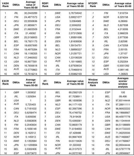
Table 5 provides us with the rankings of all the countries according to highest scores

obtained from conventional ratio and window analyses. Furthermore, looking at the rankings

according to the value added shares from manufacturing sector relative to the total economy

of the countries (VASH) we realize that Ireland and Finland have the highest performances

even though when looking at the window analysis ranking they are in the 14th (Finland) and

15th (Ireland) place. The fact that they are so high in the ranking of VASH explains the fact

that they have so high scores in terms of pure technical efficiency (Table 3).

Looking at the rankings for R&D expenditures by the total manufacturing sector

relative to the total economy (RDIP) we realize that Japan lies on the 3rd place compared to

DMUs GDW GDY Mean Variance Ranking

ESP 0 0 100 0 1

BEL 3,019 2,948 99,498 1,11131875 2

NLD 2,3 2,347 97,6514444 2,62662003 3

ITA 15,181 0,939 97,2891111 24,9333661 4

NOR 8,769 0 96,8692222 15,7898797 5

FRA 2,667 0,845 96,1966667 1,353155 6

USA 3,463 0,012 89,4097778 6,29850244 7

DEN 4,058 0,847 89,1134444 3,50342853 8

GBR 4,021 2,182 84,5118889 2,09828561 9

CAN -4,72 1,43 84,4173333 3,787293 10

SWE 9,02 1,689 71,0625556 13,7114723 11

AUS 3,622 1,682 69,7146667 5,016313 12

DEU 2,094 0,009 67,4176667 0,67695725 13

FIN -8,444 0,678 62,9504444 23,288344 14

IRL 12,902 2,279 60,5797778 25,0549984 15

the trade efficiency ranking which has the worst trade performance. Countries, which are the

last in the ranking of RDIP ratio are the most trade efficient according in the DEA window

analysis (Spain)2.

Table 5: Rankings and average values according to the ratios used and the DEA window analysis.

VASH

/Rank DMUs

Average value of Years 95-00

RDIP/

Rank DMUs

Average value of Years 95-00

NTGDP/

Rank DMUs

Average value of Years 95-00

1 IRL 30,2443289 1 SWE 3,76734542 1 FIN 7,616704

2 FIN 24,4871573 2 USA 3,09521077 2 NOR 6,325158

3 DEU 22,5550636 3 JPN 3,0364985 3 SWE 6,28069

4 JPN 21,9856671 4 DEU 2,5006202 4 NLD 5,827938

5 SWE 21,6603509 5 FRA 2,3152444 5 BEL 4,213006

6 ITA 21,49262 6 FIN 2,07312906 6 ITA 3,988228

7 GBR 20,5156603 7 GBR 1,90891696 7 DEN 3,977936

8 BEL 19,7921173 8 DEN 1,81608936 8 IRL 2,82598

9 ESP 18,6007695 9 BEL 1,59154751 9 CAN 2,473358

10 FRA 18,4975284 10 NLD 1,58890337 10 FRA 2,00105

11 CAN 18,1106355 11 NOR 1,31297721 11 JPN 1,37107

12 NLD 17,3460502 12 CAN 1,23108328 12 DEU 0,974004

13 USA 16,8977581 13 AUS 1,18116865 13 ESP 0,252354

14 DEN 16,7656618 14 IRL 0,97939034 14 GBR -0,5001392

15 AUS 13,5770863 15 ITA 0,70466916 15 AUS -0,881146

16 NOR 12,7616214 16 ESP 0,55962193 16 USA -1,36823

EXCR

/Rank DMUs

Average value of Years 95-00

IIT/

Rank DMUs

Average value of Years 95-00

Window Analysis Rank

DMUs

Averages scores/ window analysis

1 GBR 1,593832 1 BEL 89,2362129 1 ESP 100

2 IRL 1,529264 2 FRA 87,7038911 2 BEL 99,498

3 USA 1 3 GBR 86,1009596 3 NLD 97,65144444

4 AUS 0,725403 4 NLD 84,1171103 4 ITA 97,28911111

5 CAN 0,7181632 5 ESP 82,3567296 5 NOR 96,86922222

6 DEU 0,6256474 6 DEU 76,4748752 6 FRA 96,19666667

7 ITA 0,609308 7 USA 75,919439 7 USA 89,40977778

8 NLD 0,5563836 8 DEN 73,4269361 8 DEN 89,11344444

9 FIN 0,2040604 9 CAN 72,8600179 9 GBR 84,51188889

10 FRA 0,1836148 10 SWE 71,6184693 10 CAN 84,41733333

11 DEN 0,162012 11 ITA 67,428486 11 SWE 71,06255556

12 NOR 0,145913 12 IRL 64,9667409 12 AUS 69,71466667

13 SWE 0,1353584 13 FIN 64,6119426 13 DEU 67,41766667

14 JPN 0,11200894 14 NOR 61,022402 14 FIN 62,95044444

15 BEL 0,0302406 15 AUS 46,3137573 15 IRL 60,57977778

16 ESP 0,0073672 16 JPN 44,0572182 16 JPN 40,28566667

In the same lines, when we observe the exchange rate for exports for each country we

our DEA ranking and therefore they are less trade efficient compared to Belgium and Spain,

which have the lowest average exchange rate prices for exports.

Figure 2 provide us with essential information comparing overall efficiency and ratios.

More analytically we realize graphically that countries, which are more trade efficient, have,

as expected, lower exchange rates for exports. Moreover, countries with lower research and

development expenditure are more trade efficient. This is justified by the fact that most of the

goods, which are tradable, are agricultural products. Furthermore, high technology goods and

services are costly to be traded due to tariffs and taxes, which are imposed from the importing

countries. As expected countries with higher value of IIT are trade efficient.

Figure 3: Overall efficiency versus VASH; RDIP; EXCR; IIT; NTGDP and GDP

O v e ra ll E ff ic ie n c y 32 30 28 26 24 22 20 18 16 14

12 _0,2 _0,6 _1,0 _1,4 _1,8 _2,2 _2,6 _3,0 _3,4 _3,8 _4,2 0 1 2 3 4 5 6 7 8 9 10

100 80 60 40 90 85 80 75 70 65 60 55 50 45 40 100 80 60 40 8 7 6 5 4 3 2 1 0 -1 -2 9000 000 8000 000 7000 000 6000 000 5000 000 4000 000 3000 000 2000 000 1000 000 0 -100 0000

VASH RDIP EXCR

IIT NT GDP GDP

USA GBR

SW E ESP NO R NLD

JPN I TA I RL DEU FRA FI N DEN CA N BEL A US USA GBR SW E ESP

NO RNLD

JPN I TA I RL DEU FRA FI N DEN CA N BEL A US USA GBR SW E ESP NO RNLD

JPN I TA I RL DEU FRA FI N DEN CA N BEL A US USA GBR SW E ESP

NO R NLD

JPN I TA I RL DEU FRA FI N DEN CA N BEL A US USA GBR SW E ESP NO R NLD JPN I TA I RL DEU FRA FI N DEN CA N BEL A US USA GBR SW E ESP NO R NLD JPN I TA I RL DEU FRA FI N DEN CA N BEL A US

Scat t erplot of Efficiency vs VASH; RDI P; EXCR; I I T; NTGDP; GDP

These results are supported by the derived targeted values presented in table 6. These

values are obtained for the trade inefficient countries in order to become efficient. It is

noticeable that the targeted values for VASH and RDIP ratios require moderate changes for

targeted values for EXCR these are quite high. Taking Japan as an example, we realize that in

order for Japan to become trade efficient it has to reduce its exchange rates for exports

(probably making its commodities more competitive), increasing significantly the intra

industry trade and enhancing policies for trade to contribute to the country’s growth. A similar

picture is valid in the case of Australia, Canada and Great Britain while Germany, Ireland and

Italy have to reduce their exchange rates for exports, increasing their IIT ratio.

Table 6: Targeted values for the trade inefficient countries to become trade efficient

Dmus/ratios VASH RDIP EXCR IIT NTGDP AUS 12,9000 1,0318 0,6282 45,2704 -1,8017

(targeted) 12,8980 1,0313 0,3166 63,6522 3,3598

BEL 19,6071 1,6294 0,0276 91,3616 4,2639

(targeted) 19,6071 1,6294 0,0276 91,3616 4,2639

CAN 18,7393 1,3475 0,6742 75,5266 2,0036

(targeted) 18,7362 1,3478 0,3808 90,9671 4,0349

DEN 16,6914 2,1607 0,1496 75,1113 2,0172

(targeted) 16,6926 1,4218 0,1524 79,4656 4,0882

FIN 25,4403 2,4296 0,1874 62,9306 8,8126

(targeted) 25,4423 2,1561 0,1914 120,5730 6,0826

FRA 18,5611 2,1580 0,1698 88,0536 2,6523

(targeted) 17,1893 1,2474 0,3551 83,5652 3,7629

DEU 22,5416 2,5200 0,5694 77,3750 1,4948

(targeted) 24,0527 1,0068 0,1085 109,5830 1,1127

IRL 32,4701 0,8916 1,4285 61,3953 3,0235

(targeted) 26,1745 0,8977 0,0140 117,2800 0,0982

ITA 21,2019 0,6300 0,5761 68,1938 3,4049

(targeted) 18,4952 0,6343 0,0099 82,8715 0,0694

JPN 21,1880 3,3273 7,6639 46,4932 1,8352

(targeted) 21,1852 1,9259 0,6420 106,8580 6,8226

NLD 16,8322 1,5316 0,5051 84,8929 5,4151

(targeted) 16,8322 1,5316 0,5051 84,8929 5,4151

NOR 13,0402 1,1802 0,1326 59,7283 1,8959

(targeted) 13,0410 1,1151 0,1349 62,2946 3,2517

ESP 18,6643 0,6356 0,0067 83,6107 0,0672

(targeted) 18,6643 0,6356 0,0067 83,6107 0,0672

SWE 22,1579 3,7589 0,1259 72,7133 6,2853

(targeted) 22,1603 1,8678 0,1292 104,5160 5,1610

GBR 19,4651 1,9974 1,6570 85,8265 -0,9904

V. Conclusions and Policy Implications

In this study we performed an application of DEA window analysis in order to

compare international trade efficiency, by using conventional ratio measures in the suggested

model and for the time period 1996–2000. The efficiency scores and the optimal ratio levels

for inefficient countries for all the five years of the study were obtained. Results drawn from

the broadly used ratio analysis were also compared to the results derived from the DEA

window model. The advantage of using DEA compared to economic ratios is that DEA

provides us with an overall objective numerical score, ranking, and efficiency potential

improvement targets for each one of the inefficient units.

Specifically, DEA assists in efficiency comparisons with the simultaneous use of

multiple criteria, which determine efficiency for each DMU, forming a rounded judgment on

DMU efficiency taking into consideration a variety of efficiency dimensions and combining

them into a single performance measure. Looking at the results of the conventional ratio

analysis and our DEA window analysis we may conclude that even though DEA analysis

provide us with a ranking taking into account all the variables, it needs conventional ratio

analysis in order to clarify different aspects, which cannot be explained through input/output

analysis.

In our case, it seems that the trade efficient countries have clear characteristics.

Specifically, these are

- Low exchange rates. As expected, looking at the exchange rate for exports for each

country we realize that countries with higher exchange rates are the ones, which

are in the lower places of our DEA ranking, and therefore they are less trade

efficient.

- Low R&D intensity. Countries with low ranking according to their RDIP ratio are

- High value intra industry trade.

- The combination of the above mentioned factors have positive effect on the

contribution of net trade to GDP of each country.

- Countries with high ranking according to their VASH ratio have high scores in

terms of pure technical efficiency

- Scale operation does affect the trade efficiency of the country. The larger the

divergence between overall and pure technical efficiency scores the lower the

value of scale efficiency (in trade terms) and the more adverse the impact of scale

size on trade efficiency.

From the above, it can be concluded that through long-term relationships with firms

from more advanced countries, the companies from less developed countries can get access to

foreign technology, management skills and organizational expertise. Advanced countries

mainly attract efficiency- and market-seeking and asset-augmenting Foreign Direct

Investment while less developed countries are mostly attractive for resource- and

market-seeking investors.

Finally the results need to be treated with discretion and caution taking into accounts

all the economic parameters affecting trade efficiency and economic development along with

References

Asmild, M., Paradi, C., V., Aggarwall, V. and Schaffnit, C. (2004) ‘Combining DEA Window

Analysis with the Malmquist Index Approach in a Study of the Canadian Banking Industry’,

Journal of Productivity Analysis21, 67-89.

Blake, D. (1993) A short course of Economics, McGraw Hill.

Charnes, A., W., W., Cooper and E., Rhodes (1978) ‘Measuring the Efficiency of Decision

Making Units’, European Journal of Operational Research2, 429-444.

Charnes, A., Clark, C.T., Cooper, W.W. and Golany, B. (1985) ‘A Developmental Study of

Data Envelopment Analysis in Measuring the Efficiency of Maintenance Units in the U.S. Air

Forces’, Annals of Operations Research2, 95-112.

Charnes, A., Cooper, W.W. and Seiford, L.M. (1994) ‘Extension to DEA Models’, in: A.

Charnes,W. W. Cooper, A. Y. Lewin and L. M. Seiford (eds.), Data Envelopment Analysis:

Theory, Methodology and Applications, Kluwer Academic Publishers.

Coelli, T., Prasada Rao, D.S. and Battesse, E.G. (2001) An introduction to Efficiency and

Productivity Analysis, Kluwer Academic Publishers.

Halkos, G.E. and Salamouris, D.S. (2004) ‘Efficiency measurement of the Greek commercial

banks with the use of financial ratios: a data envelopment analysis approach’, Management

Accounting Research15, 201-204.

Thanasoulis, E. (2001) Introduction to the theory and application of data envelopment

analysis,Kluwer Academic Publishers.

Notes:

1

2

An economic interpretation may rely on that a country has to decide if it will be a technological leader or a

technological follower. The former case requires the involvement in expensive R and D activities. This may lead

to new inventions through patents or even to nowhere. On the other hand the technological follower has to search

for access to the technology developed by the leader. This may be achieved either by developing a similar

version but having to bear a lower R and D cost compared to the leader or by licensing the new technology from