Obstacles Avoidance Algorithm for Mobile Robots,
Using the Potential Fields Method
Vesna Antoska-Knights
1,*, Zoran Gacovski
2, Stojce Deskovski
31Faculty of Technology and Technical Sciences Veles 1400, University St. Kliment Ohridski-Bitola, Republic of Macedonia 2European University, Republic of Macedonia
3Technical Faculty, University "St. Clement Ohridski", Republic of Macedonia
Copyright©2017 by authors, all rights reserved. Authors agree that this article remains permanently open access under the terms of the Creative Commons Attribution License 4.0 International License
Abstract
In this paper - a mobile robot guidance and control has been researched in the environment full of obstacles, by using the potential fields method. The mobile robot has 4-wheels configuration, electric drive on the rear vehicles, and is directed from the front wheels (Ackerman control algorithm). A known environment has been considered, where fixed potentials were assigned to the goal and the obstacles. When the obstacles are unknown - the potential fields have to be applied, as the robot moves and detect new obstacles. A potential field’s method was applied with one attraction potential assigned to the goal point and fixed rejection points assigned to the obstacles. It moves successfully within different obstacle configurations (closely spaced obstacles), and it solves the problem with a local minimum occurrence. The simulation results showed small and stable tracking errors along 2 axes.Keywords
Mobile Robots, Guidance and Control,Trajectory Planning, Potential Fields Method, Obstacle Avoidance
1. Introduction
The autonomous robot navigation problem consists of the determining the possible path between two points, an initial and a final (goal) point. The local navigation method should produce an optimal (possibly shortest) path, avoiding the obstacles present in the moving environment. Usually, the obstacles and the target could be fixed or dynamic. The goal of the path planning method is to determine the robot’s movement, but to avoid collisions while reaching the destination. Potential fields are a good approach to the path determining problem, [1]. Different authors have undertaken different approaches to calculate appropriate field configurations.
What is the basic idea of potential fields? It is to
calculate attraction and rejection forces within the working environment of the robot to guide it to the target. The robot is treated as an object under the impact of an artificial potential field. Space is represented with an array (or field) of vectors; vectors consist of magnitude (Length of arrow) and direction (Angle of arrow). Generated robot movement is similar to a ball rolling down a hill. Goal generates attractive force, while obstacles are repulsive forces. That is the control law for the robot’s motion. A vector space will be used, as a 2D map which will be divided into squares, creating a (x,y) grid. Each element represents a square of space and perceivable objects exert a force field on the surrounding space. Other types of potential fields are: Uniform, Perpendicular and Tangential.
There are approaches that are able to produce the resultant forces required to avoid a set or several obstacles in a close distance, [4]. Several additional attractions points with flexible position and force magnitude will enable movement around big obstacles, as well as through closely placed obstacles, but the field optimization cost will be enlarged. Wu et al.[5], have successfully applied genetic algorithms, in order to optimise the potential fields with a large number of unknown obstacles and four auxiliary attraction points. Their method is rather fast and can be used for real-time control of a mobile robot.
This paper is organized as follows: in Section 2 we present the kinematic and dynamic model of the 4-wheeled mobile robot; in Section 3 - the Guidance and control method is presented, and in Section 4 - the trajectory planning algorithm using the potential field method. Finally we present the simulation results, our summary conclusions and directions for further work.
2. Mathematical Model of the Mobile
Robot
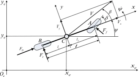
In this section, the robot movement in horizontal plane will be elaborated. A mobile robot with 4 wheels (Ackerman drive) was considered, with fixed rear wheels, and steering front wheels. Fig.2.1 shows the robot geometry while moving in 2D space. The kinematic and dynamic equations for the movement of the mobile robot can be found in [6, 7, 8], and here we’ll use these equations without derivation.
e
x e
y
e
x
e
O
x
lane centerline
χ ψ β δ
e
y C
V xk
k
y y
k
y
a
O
Figure 2.1. Kinematics of lateral vehicle motion
In many cases, when the kinematics and dynamic model of a car-like robot is required - a bicycle model is used, where front and rear vehicles are presented with a single wheel, as in Fig.2.2, [6].
The movement of the mobile robot in horizontal plane can be described as a system with 3-degrees of freedom– two translations of the mass centre (С) along
x
and yaxes, and one rotation around z axis. Three coordinate
systems are used: inertial coordinate system - fixed to the ground (global) E O x y( ; , )e e e , coordinate system fixed to the robot body (local) B C x y( ; , )and coordinate system attached to the robot trajectory K C x y( ; , )k k , where xkis axis - tangent, and ykis axis normal to the trajectory.
x
y
e y
l
e
x
ψ δ
C
x
V
y
V
e y
e
x
e
O
f l
r l
ψ
f
F
r
F D
F
B
A
β
V
Figure 2.2. Bicycle model of lateral mobile robot dynamics
The kinematic equations of the mobile robots are:
cos( )
sin( )
cos
e e
f r
x V
y V
V tg
l l ψ β ψ β β
ψ δ
= +
= +
= +
(2.1)
where: V is velocity of centre of gravity (c.g.) of the
vehicle which is at point C, ψ is yaw angle (orientation angle with respect to global coordinate xe),
β
is vehicle slip angle,χ ψ β
= + is the angle of turn of the vehicle, δ is the steering angle of front wheels,l
f and lr are distances of points A and B from centre of gravity of the vehicle, respectively,l l
= +
fl
r is wheelbase of the vehicle.Dynamic equations can be derived from Fig. 2.2 and they are:
( ) sin
( ) cos
cos
x y f D
y x f r
f f r
m V V F F
m V V F F
J l F l F
ψ
δ
ψ
δ
ψ
δ
− = − +
+ = +
= −
(2.2)
where m and J are mass and inertial moment of the vehicle around the mass centre, FD is driving force on the rear axis - along
x
axis,F
f and Fr are resultant side forces on the front and the rear wheel. The first two equations in (2.2) define the forces balance along the system axes B C x y( ; , ), while the third equation in (2.2),defines the moments’ balances around the z axis, normal to the plane Cxy.
[image:2.595.308.536.166.291.2] [image:2.595.59.286.466.627.2]tan x y r V l V l δ ψ ψ = =
, (2.3)
and their derivations have the form:
2 tan (cos ) x x y r V V l l V l
δ
ψ
δ
δ
ψ
= + = , (2.4)
Using the kinematics equations (2.1), dynamic equations (2.2), and non-holonomic connection (2.3) and its derivatives (2.4), applying some math computation, the following equations were obtained - i.e. mathematical model of the mobile robot:
(
cos
tan sin
)
e l x
x
=
ψ
−
C
δ
ψ
V
(
sin
tan cos
)
e l x
y
=
ψ
+
C
δ
ψ
V
tan x
V l
δ
ψ= (2.5)
2 2
1 [ tan (cos ) ]
x x eq D
V V J l F
d δδ δ
= +
2 2
(cos ) [ m eq(tan ) ]
d=
δ
C +Jδ
where parameters
C J
l,
eq,C
mare computed with:r l l
C l
= , Jeq =l m Jr2 + ,
C
m=
l m
2 . (2.6) The driving force FD is generated by a DC motor which rotates the rear wheels, and can be computed by:2 2
D FD D Vx x u
F
= −
C F
−
C V C u
+
, (2.7) while the parameters can be computed with:a FD a R C L = , 2 2 2 ( m b a m) w Vx
a m w
K K R b N
C
L N R
+
= , (2.8)
2 m w
u
a m w K N C
L N R =
where: Ra - resistance in armature circuit, La- inductivity in the armature circuit, Km, Kb,bm- motor constants,
w
N - number of cogs in the wheels’ gear, Nm- number of cogs in the motor axis, Rw- wheel radius.
The controller (actuator) for the steering wheels can be described as a 1-st order system:
1 1 a a c u δ δ τ = − +
(2.9)
where cais reinforcement, and τa- time constant of the actuator.
The mobile robot model obtained by the upper equations is displayed in Fig.3.2. Input in the model are the control signals u1- for front wheels control, u2- for velocity control. The output of the system is the complete state vector:
[ , , , ,
, ]
Te e x D
x y
ψ
V F
δ
=
x
(2.10)and other variables that are dependent on the robot state.
3. Robot Guidance and Control
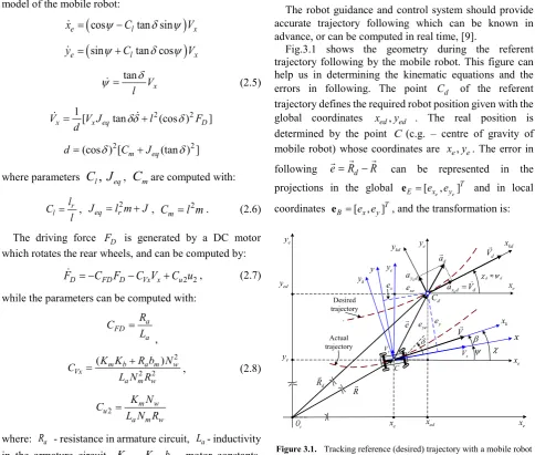
The robot guidance and control system should provide accurate trajectory following which can be known in advance, or can be computed in real time, [9].
Fig.3.1 shows the geometry during the referent trajectory following by the mobile robot. This figure can help us in determining the kinematic equations and the errors in following. The point Cd of the referent trajectory defines the required robot position given with the global coordinates x yed, ed . The real position is determined by the point C(c.g. – centre of gravity of mobile robot) whose coordinates are x ye, e. The error in following
e R
=
d−
R
can be represented in the projections in the global [ , ]e e TE = e ex y
e and in local
coordinates [ , ]T B = e ex y
e , and the transformation is:
e x e y e x e O x Desired trajectory χ ψ β δ d d
χ ≈ψ
e y C V x V y V e x e y k x d C e x d R R e d V Actual trajectory ed x ed y y e x e e y y kd x kd y xe e ye e d a k
x d d
a =V k
y d
a
k
y
Figure 3.1. Tracking reference (desired) trajectory with a mobile robot
B = BE B e T e , or
[ , ]T [ ,e e]T
x y BE x y
[image:3.595.55.540.251.662.2]В coordinate system, and is given by:
cos sin
sin cos BE = ψ = − ψψ ψψ
T T (3.2)
One way to generate the referent trajectory, given the accelerations along the trajectory tangent and normal respectively-
a
x dka
y dk , is to apply the following equations:, 0
0
(0)
, (0)
k k
d x d d d
y d
d d d
d
V a V V
a V
ψ ψ ψ
= =
= =
(3.3)
0 0 cos , (0) sin , (0)
ed d ed ed
ed d ed ed
x V x x
y V y y
ψ ψ
= =
= =
(3.4)
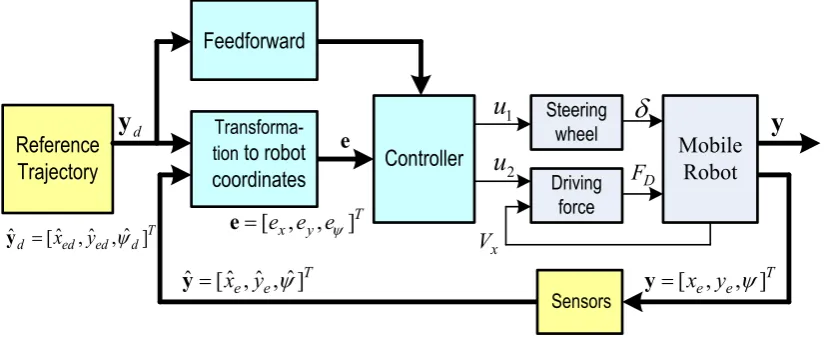
The diagram of the control system is given in Fig.3.2. The ‘Mobile robot’ block computes the equations (2.5), the block ‘Steering wheel’ solves (2.9), the block ‘Driving force’ generates the driving force – (2.7), the block ‘Transformation to robot coordinates’ computes the errors:
, ,
xe ed e
ye ed e
d
e x x
e y y
eψ
ψ
ψ
= −
= −
= −
(3.5)
transforming them in local coordinate system with (3.1), the ‘Reference trajectory’ block computes the referent trajectory. To obtain better guidance accuracy, especially when the trajectory needs fast manoeuvres, together with the feedback controller - a feedforward controller based on the inverse robot model must be applied. The controller (its algorithm) generates control signal u1 to control the steering vehicles. To generate the signal u1 - a PID controller has been used. The signal u2 defines the given velocity of the robot movement along the given trajectory. Based on the above model and the block diagram shown on Fig.3.2, a simulation model in MATLAB/Simulink was developed, which can be used for testing of the guidance algorithm. The generation of the referent trajectory in an obstacle environment is described in the following section.
Reference
Trajectory
Controller
Feedforward
Sensors
Mobile
Robot
Transforma-tion
to robot
coordinates
x
V
2u
1
u
d
y
Steeringwheely
Driving force
δ
D
F
e
ˆ
ˆ
[ , , ]
ˆ ˆ
Te e
x y
ψ
=
y
ˆˆ [ ,ˆ ˆ , ]T
[image:4.595.86.500.354.524.2]d = x yed ed ψd y
[ , , ]
T e ex y
ψ
=
y
[ , , ]
T x ye e e
ψ=
e
4. Trajectory Planning by Potential
Fields
The basic idea of trajectory planning by potential fields is very practical. Robot is presented as a point in the space and the environment is represented as a potential field, [10]. Potential field is an array of vectors which represent the space, and the vectors represent forces. Each vector consists of length of magnitude (m) and angle of arrow or direction (d).
The following equations and parameters are valid for the goal:
( , )x yG G denotes the position of the goal, ( , )x yO O denotes the position of the obstacle, d is the radius of the goal,
[ ]
, TV= x y gives the (x, y) coordinate position of the point
(robot). Distance (d) between the goal and the robot is:
(
) (
2)
2G G
D= x −x + y −y , and
(
) (
2)
2O O
D= x −x + y −y is the distance between the obstacle and the robot,
1
tan
GG
y
y
x
x
θ
=
−
−
−
- angle between the robot and the goal, α represents the strength of the attraction potential of thegoal.
Programming a single potential field - can be done by a repulsive field with linear drop-off:
0 180 = direction V D d for D d for D d D
Vmagnitude ≤>
− =
0 , (4.1)
where D is the max range of the field’s effect.
To generate potential field function U(q) for the robot - we will start with the force acting on a robot at point q:
) ( )
(q U q
F =−∇ , and environment is represented by potential function: U(x,y). Force is proportional to the
gradient of the potential function:
) , (x y U y
x =−∇ (4.2)
Environment is sum of the potential of fields, [10]: )
( ) ( )
(q U q U q
U = att + rep (4.3)
where, Uatt(q) is attracting (goal) and Urep(q) is
repulsing (obstacle) fields.
The gradient of the potential function must be differentiable: ∂ ∂∂ ∂ = ∇ y Ux U
U (4.4)
From above equations, artificial force field acting on a robot F(q), as the gradient of the potential field is given by:
)
(
)
(
q
U
q
F
=
−∇
) ( ) ( ) ( ) ( )
(q F q F q U q U q
F = att + rep =−∇ att −∇ rep (4.5)
Converting to robot control, the robot velocity is set to )
,
(vx vy , proportional to the force F(q) generated by the
field, the force field drives the robot to the goal and the robot model is derived in section 3.
Attraction potential field is defined with: 2
1
2
att attU
=
ξ
d
where d= −q qgoal ; q is the currentposition of the robot and
q
goal is the position of the attraction point;ξ
att is adjustable positive scaling factor (constant).In the attractive potential field these are the main functions: linear function of distance, quadratic function of distance and mix of the both.
Linear function of the distance is: goal att
att q q q U ( )=
ξ
−, goal goal att att att q q q q q U q F − − − = −∇ = ( ) ( ) )
( ξ (4.6)
where
ξ
att is a positive scaling factor, andq
−
q
goalis the distance.- Quadratic function of distance is given by:
2
2 1 )
( att goal
att q q q
U =ξ − (4.7)
Attracting force will converge linearly towards 0 (goal):
( ) ( )
( )
att att att goal goal
att goal
F q U q q q q q
q q
ξ ξ
= −∇ = − − ∇ −
= − − (4.8)
Repulsive potential field will generate different barriers around the obstacles: strong, if the obstacle is near, or zero - if the obstacle is far away:
0 0
0 ( )
) ( 0 1 ) ( 1 2 1 )
( ξ ρ ρ ρρ ≥≤ρρ
− = q f q if q q U rep
rep (4.9)
where ρ(q) is the minimal distance to the obstacle from
q
;ρ
0 is distance of influence of obstacle.Field is larger or equal to zero and leans to infinity, as q
approaches the obstacle:
0 0 2
0 ( )
) (
0 ( ) ( )
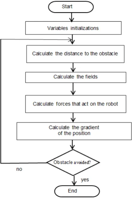
Figure 4.1. Block diagram for calculation of the potential fields
This formula is popular because it is elegant and simple. However, there could be oscillations and local minima situations with some obstacle positions, and possible problems include: trap situations due to local minima, oscillations in tight corridors, or difficultness of moving between closely spaced obstacles. Some other potential fields algorithms have been introduced in the past in order to solve these problems. Above equations for rejection forces can be modified in a case with non-reachable target when it is near the obstacles, since when the robot approaches the goal near an obstacle, the attraction force decreases and becomes drastically smaller than the increasing rejection force. The modified rejection potential takes the form of:
2
( ) 0 ( ) 0
( ) 0
1 1 1
2
0
n q
rep goal
rep q
q
d d
q q
U ξ d d d d
≤
− −
= ≥
(4.11)
For potential field path planning harmonic potentials have been used, since the robot is moving in an environment with fixed obstacles, ensuring that there are no local minima. The derived harmonic potential of the point charge q is:
2 1,3,4,...
( )
1
ln 2
n
q n r U r
q n
r
−
=
=
=
(4.12)
where 2
1
,
( , ,
1 2 n)
nr
=
∑
x x
=
x x
x
and the gradient U−∇ is described by:
1
( 2) 1,3,4,...
( )
2
r n
r q
n e n
r U r
q e n r
−
− =
−∇ =
=
(4.13)
Where
e
r denotes a unit vector in radial direction.5. Simulation Results
In accordance with the block diagram in Fig.3.2 and equations that describe each module, we developed the simulation model of the mobile robot in Matlab/Simulink. The parameters of the mobile robot which are used in the simulation are: l = 0.2540 [m] - distance between rear wheel and front wheel; b = 0.1651 [m] - space between wheels; H = 0.0762 [m] – height; D = 0.0635 [m] - diameter of wheels; F = 0.0318 [m] - width of rear wheels;
R = 0.0508 [m] - width of rear wheels; lr = 0.0889 [m] - distance from CG to rear axle; lf= 0.1651 [m] - distance from CG to front axle; Rw = 0.0318 [m] - wheel radius; m = 1.4175 [kg] - mass of the mobilniot robot; J = 0.0594 [kg*m2] - inertial moment of the robot; c
Figure 5.1. Mobile robot control system model - developed in Simulink
The first experiment for robot’s guidance and control is based on a case with a circled reference trajectory with a given radius Rd and given constant velocity along the circle
V
d . For reference trajectory generation the equations (3.3) and (3.4) were applied. In the simulation we’ve used the initial values: Vd(0) 1m/s= ,(0) 0rad
d
ψ
= , xed(0) 0m= , yed(0) 0m= . The tangentacceleration of the vehicle is аx dk =0 m/s, and the normal
(centripetal) acceleration for Rd =10m and Vd =1m/s
is 2/ 0.1m/s2
k
y d d d
а =V R = . The initial conditions for the mobile robot are: xe(0) 0m= , ye(0) 0m= ,
(0) 0rad
ψ
= Vx(0) 0.5m/s= , FD(0) 0 N= ,(0) 0rad
δ
= . Simulation results for the robot’s motion along circular trajectory are given in Fig.5.2 to Fig.5.7.Fig. 5.2 shows the robot movement along circular trajectory with Rd =10m. Fig.5.3 shows the course angle change during the motion along the reference trajectory, as well as the error of following.
Figure 5.2. Mobile robot movement along circled referent trajectory
Figure 5.3. Robot course angle following during the movement along circular referent trajectory
Figures 5.4, 5.5 represent the errors of trajectory following along the xk ,yk axes attached to the robot trajectory K C x y( ; , )k k .
Figure 5.4. Tracking error along хk axis
-10 -5 0 5 10
0 5 10 15 20
25 Nominal and Actual Trajectories
xe [m]
ye [
m
]
Nominal traj. Actual traj.
0 20 40 60 80 100 120 140 160
-2 0 2 4 6 8 10 12 14 16
Referent ψd and actual ψ course angles, tracking error eψ
t [s]
ps
id
[r
ad
], p
si
[r
ad
], e
ψ
[r
ad]
ψd ψ
eψ
0 20 40 60 80 100 120 140 160
-0.16 -0.14 -0.12 -0.1 -0.08 -0.06 -0.04 -0.02 0 0.02
0.04 Error exk=xkd-xk
t [m]
ex
k [
m
[image:7.595.309.523.253.425.2] [image:7.595.79.258.521.722.2] [image:7.595.307.523.526.718.2]Figure 5.5. Tracking error along yk axis.
[image:8.595.58.278.81.285.2]Fig. 5.6, 5.7 show the change of the nominal and actual coordinates of the robot relatively to the global inertial (coordinate) system С О x y( ; , )е е , as well as the errors in following.
Figure 5.6. Nominal and actual coordinates and tracking error along xe
[image:8.595.311.538.197.648.2]axis.
Figure 5.7. Nominal and actual coordinates and tracking error along ye
axis.
In the next experiment we have simulated the robot motion in the obstacle environment. Referent trajectory in an obstacle environment is generated in the block Reference Trajectory Generator using potential field method. Fig. 5.8 shows how the mobile robot follows this referent trajectory. The obstacles in Fig.5.8 are presented by circles.
Fig 5.9 represents the robot course angle following during the movement along the referent trajectory.
Figure 5.8. Referent trajectory following
d
ψ
- nominal angle, ψ- real angle, eψ tracking errorFigure 5.9. Robot course angle following during the movement along referent trajectory
0 20 40 60 80 100 120 140 160
-0.16 -0.14 -0.12 -0.1 -0.08 -0.06 -0.04 -0.02 0 0.02
0.04 Error exk=xkd-xk
t [m]
ex
k [
m
]
0 20 40 60 80 100 120 140 160
-10 -5 0 5 10
15 Nominal and Actual xe Coordinates, and error exe
t [m]
xed,
x
e [
m
]
Nominal xed Actual xe Error exe
0 20 40 60 80 100 120 140 160
-5 0 5 10 15 20
25 Nominal and Actual ye Coordinates, and error eye
t [m]
yed,
y
e,
ey
e [
m
]
Nominal yed Actual ye Error eye
0 10 20 30 40 50 60 70 80 90 100
0 10 20 30 40 50 60 70 80
90 Nominal and Actual Trajectories
xe [m]
ye [
m
]
Nominal traj. Actual traj.
0 20 40 60 80 100 120 140 160 -1
-0.5 0 0.5 1 1.5 2
Referent ψd and actual ψ course angles, tracking error eψ
t [s]
ps
id
[r
ad
], p
si
[r
ad
], e
ψ
[r
ad] ψ
d
[image:8.595.309.535.203.427.2] [image:8.595.63.278.357.532.2] [image:8.595.64.277.565.731.2]Figure 5.10. Trajectory following along х axis
Figure 5.11. Trajectory following along y axis
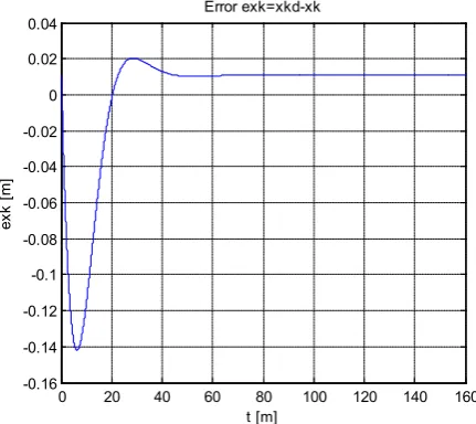
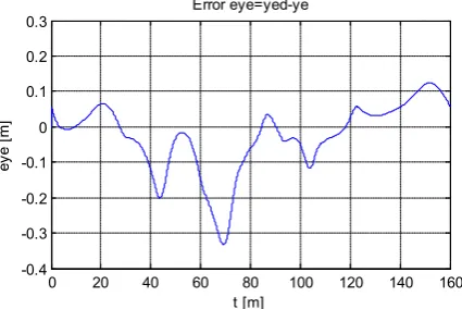
[image:9.595.63.278.93.406.2]Fig.5.10, and Fig.5.11 present trajectory following along x, and y axes, respectively. Tracking errors along xeand ye axes are given in Fig.5.12 and Fig.5.13 respectively.
Figure 5.12. Tracking error along хe axis
Figure 5.13. Tracking error along yeaxis
6. Conclusions
In this paper - the mobile robot guidance and control was researched - in the environment full of obstacles, by using the potential field’s method. The mobile robot has 4-wheels configuration, electric drive on the rear vehicles, and is directed from the front wheels (Ackerman control algorithm). We have simulated a movement in a horizontal (2D) plane and the robot is modelled as a 3-DOF system (three degrees of freedom).
Our method uses functions defining potential fields at its position to calculate component vector. Only a part of the field that affects the robot is computed for each behaviour of the potential field; the sum of the vectors at the robot’s position gave the resultant output vector. We did not have issues with combining potential fields; the influence of the low update rates are the broken (irregular) paths.
The contribution of this work (in comparison to other authors) is that we have simulated real 4-wheel robot with complete kinematics and dynamics, unlike existing works, which consider single mass point. The robot was treated as a mass object, it could not to change velocity and direction instantaneously (cannot happen). We found a solution for local minimum problem; if the global minimum is not guaranteed, we have chosen the functions in such a way that global minimum can be guaranteed and the robot will escape the local minima. Previous behaviours that should be avoided are included – thus we track where robot has been and we lead the robot to other places. These “avoid” behaviours will define desired direction and will insert tangential fields around the obstacles.
The tracking errors along both axes remain low (close to zero) and the time to stabilize is in terms of seconds (comparable to previous works, [11]).
0 20 40 60 80 100 120 140 160 0
20 40 60 80
100 Nominal and Actual xe Coordinates, and error exe
t [m]
xed,
x
e [
m
]
Nominal xed Actual xe Error exe
0 20 40 60 80 100 120 140 160
-20 0 20 40 60 80
100 Nominal and Actual ye Coordinates, and error eye
t [m]
yed,
y
e,
ey
e [
m
]
Nominal yed Actual ye Error eye
0 20 40 60 80 100 120 140 160
0 0.05 0.1 0.15 0.2 0.25 0.3
0.35 Error exe=xed-xe
t [m]
ex
e [
m
]
0 20 40 60 80 100 120 140 160
-0.4 -0.3 -0.2 -0.1 0 0.1 0.2
0.3 Error eye=yed-ye
t [m]
ey
e [
m
[image:9.595.62.279.481.628.2]REFERENCES
[1] Shimoda S., Kuroda Y., Iagnemma K., (2005), Potential field navigation of high speed unmanned ground vehicles on uneven terrain, IEEE Int. Conf. on Robotics and Automation, Barcelona, Spain, pp.2828-2833.
[2] Khatib O. (1990), Real-time obstacle avoidance for manipulators and mobile robots, In Autonomous Robot Vehicles, (Edited by I.J. Cox and G.T. Wilfong), pp. 396-404, Springer-Verlag.
[3] Rimon E., Koditschek D. (1992). Exact Robot Navigation using Artificial Potential Functions. IEEE Trans. on Robotics and Automation, pp. 501-517, October (1992). [4] Borenstein J. and Koren Y. (1991), The vector field
histogram-fast obstacle avoidance for mobile robots, IEEE Transactions on Robotics and Automation 7, pp.278-288. [5] Wu K.H., Chen C.H., and Ko J.M, (1999). Path planning and
prototype design of an AGV. Mathematical and Computer Modelling, vol.30, pp.147-167.
[6] Rajamani R. (2011). Vehicle Dynamics and Control, Second Edition, Springer - New York, Dordrecht, Heidelberg, London.
[7] Siegwart R., I. R. Nourbakhsh, D. Scaramuzza, (2011). Introduction to Autonomous Mobile Robots, Second Edition,
A Bradford Book The MIT Press Cambridge, Massachusetts London, England.
[8] Tzafestas G. S. (2014). Introduction to Mobile Robot Control, Elsevier, 32 Jamestown Road, London NW1 7BY. [9] Cook G., (2011). Mobile Robots: Navigation, Control and
Remote Sensing, A John Wiley & Sons, Inc., Publication. [10]Robotin R., Lazea G., Herle S. (2004). Hybrid Goal
Acquisition System for Pioneer 2 Mobile robot. Journal of Control Engineering and Applied Informatics (CEAI), vol. 6, no. 2, pp. 51-54.
[11]Kozłowski K., D. Pazderski, I.Rudas, J.Tar, (2004). Modeling and control of a 4-wheel skid-steering mobile robot: From theory to practice, Polish-Hungarian Bilateral Technology Co-operation Project and statuary grant No. DS 93/121/04 of Poznan University of Technology. [12]Moret, E. N. (2003). Dynamic Modeling and Control of a
Car-Like Robot, Master Thesis, Virginia Polytechnic Institute and State University.