Assessment of Cooling System Reliability based on its Success Criteria during Transient Condition

Assessment of Cooling System Reliability based on its

Success Criteria during Transient Condition

Akram W.Ezzat,

Engineering University of Baghdad

Salah S. Abed-Alkareem,

Ph.D.

Department of Machines and Agriculture Equipment

Engineering University of Baghdad

Iman Q. Al Saffar

Department of Mechanical Engineering University of Baghdad

ABSTRACT

Evaluation of cooling system reliability of any heat generation system has important impact on system engineering safety during transient conditions. Loss or reduction of flow is the main transient initiating event that leads to reduction in heat transfer ability of the cooling system.

The research target is to evaluate the reliability of typical cooling system theoretically based on its success criteria during both steady & transient states. It emphasis on analytical approach to fix the main success criteria of cooling system based on calculated heat transfer parameters during flow reduction transient, while it use the probabilistic approach for evaluating overall system reliability based on this success criteria. Four types of design layout is specified during this study which fulfill cooling system design criteria during postulated cooling deficiency that leads to sequential local or nucleate boiling on heat resource surface and extends to film boiling and boiling crisis later on.

System reliability calculations are conducted for two types of success criteria. The first is based on 75% of full cooling capacity, while the second requires 50% of full cooling capacity for each type of design layout which ensures minimum cooling requirements during above mentioned transient conditions. The results show the effect of redundant pumping branches increase on the overall system reliability during steady state operation. It investigates further system reliability versus redundancy percentage based on the number of cooling system branches required for each design type during transient condition based on its success maintain certain acceptable temperature on heat source surface during transient conditions.

Keywords

Reliability, success criteria, flow reduction transient, nucleate and film boiling.

1.

INTRODUCTION

Several researches have been conducted to estimate cooling system reliability based on deterministic approach which deals directly with the boiling safety margins as design criteria during both steady and transient conditions.

Qing Lu et al. 2009 [1], investigated the course of the partial and total blockage of a channel in the IAEA 10 MW MTR pool type research reactor core without scram. The analysis was performed with best estimate code RELAP5/MOD3.3. The interaction of the obstruction channel and its adjacent channels has been taken into account. The results indicated that even when the flow channel has been totally blocked,

there is still no boiling occurrence, and the fuel temperature is low enough to maintain its integrity. Hainoun et al. 2010 [2], used the thermal hydraulic code MERSAT, (Model for Evaluation of Reactor Safety and Analysis of Thermal hydraulic) in his study. Detailed model including primary and secondary loop was developed for the International Atomic Energy Agency, IAEA reference research reactor material MTR 10MW. The developed model enables the simulation of expected neutronic and thermal hydraulic phenomena during normal operation, reactivity and loss of flow accidents. They found that two different losses of flow accident have been simulated using slow and fast decrease time of core mass flow rate. In both cases the expected flow reversal from downward forced to upward natural circulation has been successfully simulated. His results indicated that in accidents the limit of onset of sub-cooled boiling was not arrived and consequently no exceed of design limits in term of thermal hydraulic instability or DNB is observed. Hong Gao and Xuewu Cao 2011[3], developed a mathematical model for solving flow rate transient and pump speed transient during flow coast down period. The flow rate and pump speed solved analytically. The calculated non-dimensional flow rate and non-dimensional pump speed using the model compared with published experimental data of two nuclear power plants and a reactor model test on flow coast down transient. The comparison results showed a good agreement. As the flow rate approaches to zero, the difference between experimental and calculated values increases due to the effect of mechanical friction loss.

(OFI) that encounter the downward flow direction at low pressure and low velocity system (LPLV). It’s also conclude that the elapsed time required for the surface temperature to reach its steady state values after each transient scenario is less than that related to bulk water temperature as long as the water temperature kept below its saturation temperature. L. Burgazzi [5] investigated in his research reliability based design approach based on thermal – hydraulic thermal system. The concept of functional failure, i.e possibility that the heat will exceed the capacity in reliability frame work in terms of performance parameter is introduced by the author for the reliability evaluation of a natural circulation passive system, designed for decay heat removal of innovative light water reactor. Water flow rate circulating is selected as passive system performance characteristic parameter and the related limit state or performance function is defined. The probability of system failure is assessed in terms of safety margin, corresponding to the LSF. Results obtained from the research help the designer to determine the allowable limits or set the safety margin for the system operation parameters, to meet the safety and reliability requirements.

2.

THEORETICAL ASSUMPTIONS

AND CALCULATIONS

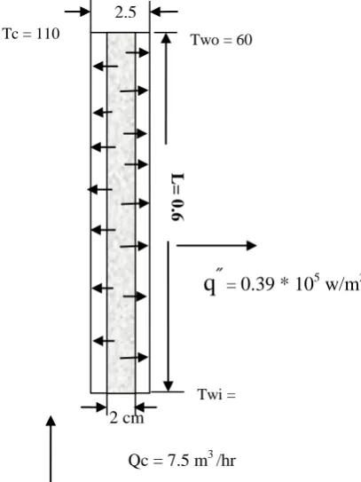
The heat generation system consists of heat source that produce 147.7 KW heat power. The heat source consist of 100 heating elements, each element is cooled by water inside an annulus between its outer surface and the water channel that contain the heating element as shown in figure (1). The total water flow rate in the cooling system required to cool the heat source is (6.4 m3/hr), which ensures water velocity inside each cooling channel of 0.1 m/s.

Taking into account the friction losses in the system and flow control valve reduction ratio the cooling system design criteria requires 7.5 m3/hr water flow rate during normal steady state condition. Fuel element and water channel dimensions are shown in figure (1).

Steady state operation, Case (1):

The following equations show the heat and mass balance for each cooling channel during steady state condition;

Ah = 0.6 * π (0.02) = 3. 77 * 10-2 m2 Af = [(2.5 *10-2)2] * = 1077 * 10-4 m2 V = 0.1 m/s

e

ṁ = ρ v A f

103 * 0.1 *1.77 * 10-4 = 1.77 * 10-2 kg ṁ t = 1.77 * 10-2 * 102 = 1.77 kg/ s

ṁ t = 1.77 kg/s * m3/103 kg * 3600s/ hr = 6.4 m3/hr

h= 0.021 ρ G (1+2.3De/L) / [(De G /µ)0.2 Prf 0.66(µw/ µb)0.14]

h= 778 w/m2 Where:

De =5 * 10-3, µ = 8.6x10-4, Pr =5.85 Qe = Qt/100 = 147.4x1000/100 = 1474 w

q'' = 1474 /(3.77x10-2)= 3.9x104 w/m2

∆Tw = Q/ m Cp= 1474 /(1.77x10-2x4170) = 20oC

Two = 40 + 20 = 60

Tco = Two + q" /h = 60 + 3.9x104/778 = 120oC

Under full cooling system pressure, the local pressure in the thermal outlet ensures water sub cooled state near the heating surface.

Transient Conditions:

Case (2): (75% of full capacity)

V = 0.075 m/s, Tco = 129.6 , Two = 66.5

The postulated transient case ensures heating surface temperature above the water saturation temperature based on its local pressure which in turn leads to nucleate boiling that may extend to film boiling in case if it is not mitigated. Case (3): (50% of full capacity)

V = 0.05 m/s, Tco = 167OC

The postulated transient case ensures bulk water temperature close from water saturation temperature based on estimated two phase heat transfer coefficient.

Design types considered in the calculations: Cooling system water flow rate, Qp =7.5 m3 /hr

A. 1 pump ⇒ each 7.5 m3 /hr B. 2 pumps ⇒ each 3.75 m3 /hr C. 3 pumps ⇒ each 2.5 m3 /hr D. 4 pumps ⇒ each 1.875 m3 _/hr

Case 1: To reach Full Capacity (Qp = 7.5 m3 _/hr) A. Use (2) pumps ⇒ s.c = 1/2

B. Use (3) pumps ⇒ s.c = 2/3 C. Use (4) pumps ⇒ s.c = 3/4 D. Use (5) pumps ⇒ s.c = 4/5

Qc = 7.5 m3 /hr 2 cm

Tc = 110 _{Two = 60}

2.5 cm

L

=

0

.6

m

Twi = 40

q

˝

0.39 * 10

w/m

Temperature Sensing F

RL1

RL2

RL3

RL4

RL5

RPL1

RPL2

RPL3

RPL4

RPL5

RV11 RP1 RV12

RV51 RP5 RV52

Heat Source

Flow Control Interlock

RIC RSE

Flow Direction Case 2: To reach 75% Capacity (Qp = 5.625 m3 _/hr)

A. Use (2) pumps ⇒ s.c = 1/2 B. Use (3) pumps ⇒ s.c = 2/3 C. Use (4) pumps ⇒ s.c = 3/4 D. Use (5) pumps ⇒ s.c = 3/5

Case 3: To reach 50% Capacity (Qp = 3.75 m3 /hr) A. Use (2) pumps ⇒ s.c = 1/2

B. Use (3) pumps ⇒ s.c = 1/3 C. Use (4) pumps ⇒ s.c = 2/4 D. Use (2) pumps ⇒ s.c = 2/5

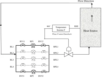
The cooling system consists of temperature sensing and flow controlling system which initiates and control the pumping branches used to cool the heat source and ensure steady state cooling requirements and keep heat source surface temperature below saturation temperature of the adjacent coolant to avoid nucleate boiling on its surface which may proceeds to film boiling during transient conditions.

Four types of design are chosen for analysis. Each of it has design criteria that ensure steady state safe operation during normal conditions and it has also to fulfill heat source integrity for a postulated period during transient conditions based on 75% of cooling system capacity and to withstand film boiling influence on heat removal by ensuring heat source integrity for additional time margin based on 50% of cooling capacity.

The design criteria of the cooling system is based on maximum (8) continuous operation hours per day during steady state operations while the transient condition requires certain time margin for 75% and 50% cooling system capacity to ensure system safety during transient condition. Due to special safety requirements of the heat generation system the cooling system operation and maintenance requirement refers to complete preventive test and maintenance on daily basis to return back system reliability to its original values during this mention period, each pumps line is isolated using the upstream for downstream valves.

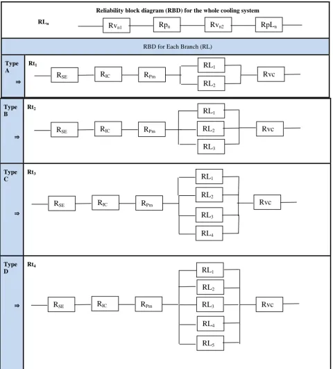
Figure (2) shows system layouts for 4 design types while figure (3) illustrates the reliability block diagram for each system type. For the purpose of overall system reliability evaluation the reliability of each branch is estimated first using the following general equation which depends on the number of branches k that are required to success out of the total number of branches for each case, (design type), n. Rb(k, n, r) = ∑n r=k (rn) Rik(1 – Ri)n-r

Where:

n: is the minimum number of lines in each case per each type of design

k: is the minimum number of branches required for system success

R : is the reliability of each branch

Note that this equation will be used for each system type based on their different success criteria. Figure (3) shows the reliability block diagram for the whole cooling system, RDB.

Reliability block diagram (RBD) for the whole cooling system

RLn

RBD for Each Branch (RL)

Type A

⇒

Rt1

Type B

⇒

Rt2

Type C

⇒

Rt3

Type D

⇒

Rt4

Figure 3: Reliability block diagram, RDB for the four cooling systems types

RLn = Rvn1. Rpn. Rvn2. Rpln Where:

n= 1, 2 for system type (A) n= 1, 2, 3 for system type (B) n= 1, 2, 3, 4 for system type (C) n= 1, 2, 3, 4, 5 for system type (D)

3. RESULTS AND DISCUSSION

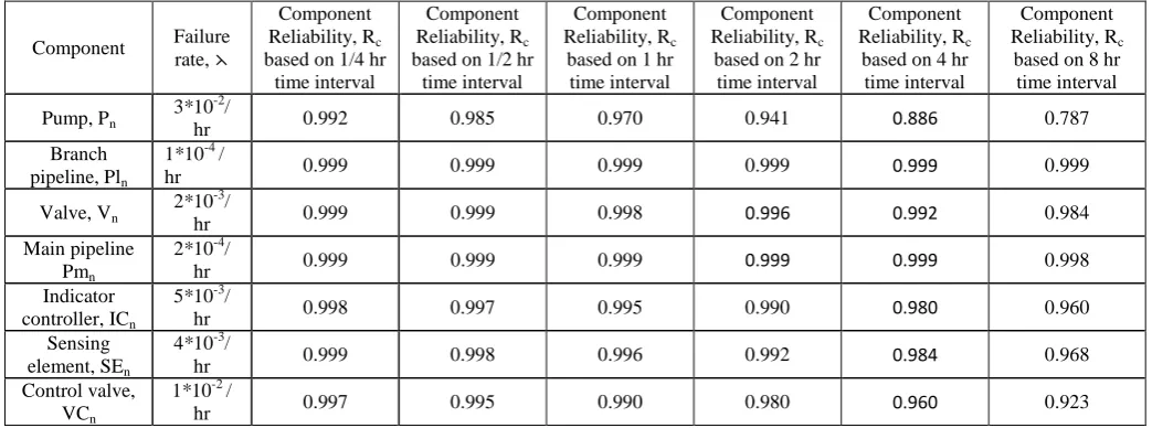
The reliability of cooling system components is estimated based on their failure rates using typical data for different mission times. Table (1) shows the failure rates and the estimated reliability of each component.

Rv

Rp

Rv

RpL

R

R

R

RL

RL

Rvc

R

R

R

RL

RL

Rvc

RL

R

R

R

RL

RL

Rvc

RL

RL

RL

RL

RL

R

R

R

RL

Table (1): System equipment reliability based on their failure rates during steady state and both cases of transient states.

Component Failure rate, ⋋

Component Reliability, Rc

based on 1/4 hr time interval

Component Reliability, Rc

based on 1/2 hr time interval

Component Reliability, Rc

based on 1 hr time interval

Component Reliability, Rc

based on 2 hr time interval

Component Reliability, Rc

based on 4 hr time interval

Component Reliability, Rc

based on 8 hr time interval Pump, Pn

3*10-2/

hr 0.992 0.985 0.970 0.941 0.886 0.787

Branch pipeline, Pln

1*10-4 /

hr 0.999 0.999 0.999 0.999 0.999 0.999

Valve, Vn

2*10-3/

hr 0.999 0.999 0.998 0.996 0.992 0.984

Main pipeline Pmn

2*10-4/

hr 0.999 0.999 0.999 0.999 0.999 0.998

Indicator controller, ICn

5*10-3/

hr 0.998 0.997 0.995 0.990 0.980 0.960

Sensing element, SEn

4*10-3/

hr 0.999 0.998 0.996 0.992 0.984 0.968

Control valve, VCn

1*10-2 /

hr 0.997 0.995 0.990 0.980 0.960 0.923

Typical calculation procedure for estimation the reliability of different cooling system types for different success criteria during normal operation mode based on (8) hours continuous operation is shown below.

Type (A) System Design:

For such type of system the expected operation modes during steady state and transient cases are based on the number of branched required to be ready during these cases which are 0/2 and 1/2.

RsA, 0 / 2⇒ RSE. RIC . RPm. (RL1, RL2) 0 / 2. Rvc RLn = 0.984 * 0.787 * 0.984 * 0.999 = 0.761

Where: (RL1, RL2)0/2=∑

2 r=0 (0

2

) RLnr(1 – RLn)2-r

(RL1, RL2) 0/2 = (1 – RLn)2 + 2 RLn (1- RLn) + RLn2 Thus;

RsA , 0 /2⇒ 0.968 * 0.96 * 0.998 * [(1 – 0.761)2 +2*(0.761)* (1 – 0.761) + (0.761)2 _{] * 0.923 = 0.856}

RsA, 1/2⇒ RSE. RIC . RPm. (RL1, RL2) 1/2. Rvc RLn = 0.984 * 0.787 * 0.984 * 0.999 = 0.761

Where: (RL1, RL2)1/2=∑

2 r=1 (1

2

) RLnr(1 – RLn)2-r (RL1, RL2) 1/2 = 1- [(1 - RL1)* (1- RL2)]

Thus;

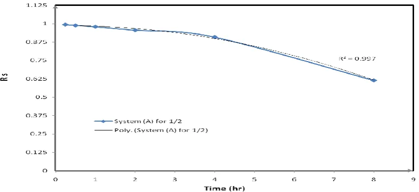
RsA, 1/2⇒ 0.968 * 0.96 * 0.998 * [1 – (1 – 0.761)2] * 0.923 = 0.841

Type (B) System Design

For such type of system the expected operation modes during steady state and transient cases are based on the number of branched required to be ready during these two cases which are 1/3 and 2/3.

RsB,1/3⇒ RSE. RIC. RPm. (RL1, RL2, RL3) 1/3 . Rvc RLn = 0.984 * 0.787 * 0.984 * 0.999 = 0.761 Where:

(RL1, RL2, RL3)1/3=∑3 r=1 (13) RLnr(1 – RLn)3-r

(RL1, RL2, RL3) 1/3 = 3 RLn (1- RLn) 2 +3 RLn2* (1- RLn) +

RLn3

Thus;

RsB,1/3 ⇒ 0.968 * 0.96 * 0.998 * [3 * (0.761) * (1-0.761)

2

+3 * (0.761)2 * (1-0.761) + (0.761) 3 ]* 0.923 = 0.844

RsB,2/3⇒ RSE. RIC. RPm. (RL1, RL2, RL3) 2/3 . Rvc RLn = 0.984 * 0.787 * 0.984 * 0.999 = 0.761 Where:

(RL1, RL2, RL3)2/3=∑3 r=2 (23) RLnr(1 – RLn)3-r

(RL1, RL2, RL3) 2/3 = 3 RLn2 * (1- RLn)1+ RLn3 * (1- RLn)0 Thus;

RsB,2/3 ⇒ 0.968 * 0.96 * 0.998 * [3 * (0.761)2 * (1-0.761) + (0.761)3]* 0.923 = 0.732

Type (C) System Design

For such type of system the expected operation modes during steady state and transient cases are based on the number of branched required to be ready during these cases which are 1/4 , 2/4 and 3/4.

RsC,1/4⇒ RSE * RIC * RPm * (RL1, RL2, RL3, RL4) 1/4* Rvc RLn = 0.984 * 0.787 * 0.984 * 0.999 = 0.761

Where:

(RL1, RL2, RL3, RL4)1/4=∑4 r=1 (14) RLnr(1 – RLn)4-r

(RL1, RL2, RL3, RL4) 1/4= 4* RLn* (1- RLn)3 + 6* RLn2* (1-

RLn)

2 +4 RLn

3 *

(1- RLn)+ RLn4

Thus;

RsC,1/4 ⇒0.968 * 0.96 * 0.998 * [4* (0.761) * (1-0.761)3 +6 * (0.761)2 * (1-0.761) 2 + 4* (0.761)3 * (1-0.761) + (0.761)4 ]* 0.923 = 0.853

RsC,2/4⇒ RSE. RIC. RPm. (RL1, RL2, RL3, RL4) 2/4. Rvc RLn = 0.984 * 0.787 * 0.984 * 0.999 = 0.761

(RL1, RL2, RL3, RL4)2/4=∑4 r=2 (24) RLnr(1 – RLn)4-r

(RL1, RL2, RL3, RL4) 2/4= 6* RLn2* (1- RLn)2 + 4* RLn3* (1-

RLn) + RLn4

Thus;

RsC,2/4 ⇒ 0.968 * 0.96 * 0.998 * [6 * (0.761)

2

* (1-0.761)2 +4 * (0.761)3 * (1-0.761) + (0.761)4 ]* 0.923 = 0.818

RsC,3/4⇒ RSE. RIC. RPm. (RL1, RL2, RL3, RL4) 3/4. Rvc RLn = 0.984 * 0.787 * 0.984 * 0.999 = 0.761

Where:

(RL1, RL2, RL3, RL4)3/4=∑4 r=3 (34) RLnr(1 – RLn)4-r (RL1, RL2, RL3, RL4)3/4 = 4* RLn

3

* (1- RLn) + RLn4 * (1- RLn)0

Thus;

RsC,3/4⇒0.968 * 0.96 * 0.998 * [4 * (0.761)3 * (1-0.761) + (0.761)4 *

(1-0.761)0]* 0.923 = 0.648 Type (D) System Design

For such type of system the expected operation modes during steady state and transient cases are based on the number of branched required to be ready during these cases which are 2/5, 3/5 and 4/5 .

RsD,2/5 ⇒ RSE* RIC *RPm * (RL1, RL2, RL3, RL4, RL5) 2/5* Rvc RLn = 0.984 * 0.787 * 0.984 * 0.999 = 0.761

Where:

(RL1, RL2, RL3, RL4, RL5)2/5=∑ 5

r=2 (2 5

) RLnr(1 – RLn)5-r (RL1, RL2, RL3, RL4, RL5) 2/5 = 10* RLn2 * (1- RLn)3+ 10* RLn3 * (1- RLn) 2 + 5 RLn4 * (1- RLn) + RLn5

Thus;

RsD,2/5 ⇒0.968 * 0.96 * 0.998 * [10 * (0.761)2 * (1-0.761)3 +10* (0.761)3 * (1-0.761) 2 + 5 (0.761)4 * (1- 0.761) + (0.761)5] * 0.923 = 0.845

RsD,3/5⇒ RSE* RIC *RPm * (RL1, RL2, RL3, RL4, RL5) 3/5* Rvc RLn = 0.984 * 0.787 * 0.984 * 0.999 = 0.761

Where:

(RL1, RL2, RL3, RL4, RL5)3/5=∑ 5

r=3 (3 5

) RLnr(1 – RLn)5-r (RL1, RL2, RL3, RL4, RL5) 3/5 = 10* RLn3 * (1- RLn)2+ 5* RLn4 * (1- RLn) + RLn5

Thus;

RsD,3/5 ⇒ 0.968 * 0.96 * 0.998 * [10 * (0.761)3 * (1-0.761)2 +5* (0.761)4 * (1-0.761) + (0.761)5] * 0.923 = 0.777

RsD,4/5 ⇒ RSE* RIC *RPm * (RL1, RL2, RL3, RL4, RL5) 4/5* Rvc RLn = 0.984 * 0.787 * 0.984 * 0.999 = 0.761

Where:

(RL1, RL2, RL3, RL4, RL5)4/5=∑ 5

r=4 (4 5

) RLnr(1 – RLn)5-r (RL1, RL2, RL3, RL4, RL5) 4/5 = 5 RLn4 * (1- RLn)1 + RLn5 * (1- RLn) 0

Thus;

RsD,4/5 ⇒0.968 * 0.96 * 0.998 * [5 * (0.761)4 * (1-0.761)1 + (0.761)5 *

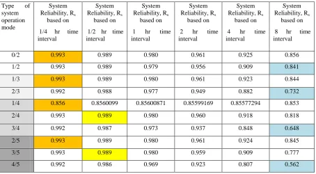
(1-0.761)0] * 0.923 = 0.562

Table (2) shows the reliability of different system types based on their success criteria and operation mission time. The first column refers to the adopted success criteria for system type. The white cells in the first column refers to success criteria of system type A, light gray cells refers to success criteria of system type B, moderate gray refers to success criteria of system type C while those related to system type D are colored by dark gray.

Table 2: System types reliability based on their success criteria and operation mission time

Type of system operation mode

System Reliability, Rs

based on 1/4 hr time interval

System Reliability, Rs

based on 1/2 hr time interval

System Reliability, Rs

based on 1 hr time interval

System Reliability, Rs

based on 2 hr time interval

System Reliability, Rs

based on 4 hr time interval

System Reliability, Rs

based on 8 hr time interval

0/2 0.993 0.989 0.980 0.961 0.925 0.856

1/2 0.993 0.989 0.979 0.956 0.909 0.841

1/3 0.993 0.989 0.980 0.961 0.923 0.844

2/3 0.992 0.988 0.977 0.949 0.882 0.732

1/4 0.856 0.8560099 0.85600871 0.85599169 0.85577294 0.853

2/4 0.993 0.989 0.980 0.960 0.918 0.818

3/4 0.992 0.987 0.973 0.937 0.848 0.648

2/5 0.993 0.989 0.980 0.961 0.924 0.845

3/5 0.993 0.989 0.980 0.959 0.909 0.777

4/5 0.992 0.986 0.969 0.923 0.807 0.562

As mentioned before system reliability during normal operation is based on full system capacity for continuous (8) hours operation. System reliability during transient condition based on 75% system capacity which leads to nucleate boiling on the heat source surface is estimated based on 30 minutes mission time while system reliability during transient condition that leads to film boiling during 50% system capacity operation mode is estimated based on 15 minutes mission time.

During steady state operation the system needs all their components including their branches based on the adopted success criteria. Such systems reliabilities are highlighted by blue color in last column of table (2) for (8) hour continuous operation mode. Figure (8) shows the relationship between system reliability and the redundant percentage RD% for each system design type. RD% refers also to the additional cost percentage during such adopted design.

Where:

Number of cooling branches available for such design type

RD% = ---

Number of cooling branches required to fulfill steady state operation

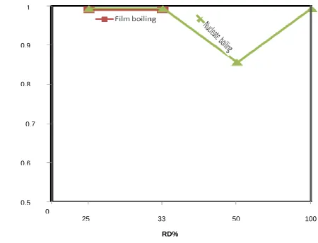
During transient operation condition that leads to nucleate boiling the system needs all their components including their branches based on adopted success criteria highlighted by yellow colors shown in table (2) for minimum half an hour continuous operation mode. It is clear that for short times system reliability is not affected by the success criteria of each system design type. During transient operation condition that leads to film boiling the system needs all their components including their branches based on adopted success criteria highlighted by orange colors shown in table (2) for minimum quarter hour continuous operation mode. Same conclusion is reached regarding the minor effect of system design types on system reliability due to the short mission time. Figures (8&9) show the relation between system reliability and redundant percentage during both steady state and transient conditions.

4.

CONCLUSIONS

It could be concluded that during steady state operation as system redundancy percentage increases its reliability increases but this reliability saturates at high redundant values, which means that system types C&D are more optimum than the other types. It is also clear that during transient conditions design types A&B does not pass through the nucleate boiling phenomena rather than it passes directly from normal operation mode to film boiling case which could be regarded as considerable drawback in addition to the extra cost of such type of systems estimated from their redundant percentage versus minor reliability enhancement gained from such types of cooling system designs. Accordingly optimum system design is adopted based on its reliability enhancement versus system cost which is related to its redundant percentage.

5.

ACKNOWLEDGEMENT

Dr. Ezzat A. W acknowledges SRF – IIE and American University MADABA, AUM for its assistance to accomplish this work.

6. REFERENCES

[1] Qing Lu, Suizheng Qiu, G.H. Su., 2009 "Flow blockage analysis of a channel in a typical material test reactor core" Journal of Nuclear Engineering and Design, Vol. 239, pp. 45-50.

[2] Hainoun, N.Ghazi, B. Mansour Abdul-Moaiz., 2010 "Safety analysis of the IAEA reference research reactor during loss of flow accident using the code MERSAT" Journal of Nuclear Engineering and Design, Vol. 240, pp.1132-1138.

[3] Hong Gao, Feng Gao, Xianchao Zhao, Jie Chen, Xuewu Cao. 2011) "Transient flow analysis in reactor coolant pumping systems during flow coast down period", Journal of Nuclear Engineering and Design, Vol. 241, pp.509-514.

[4] A. W. Ezzat, S. I. Hasan, 2013, “Thermal analysis of immersed heat source during flow reduction transient” , International journal of computer applications, Vol. 83, No.6, pp. 0975-8887.

[5] L. Burgazzi, 2006, Thermal hydraulic passive system reliability based design approach, Reliability engineering and system safety, Vol. 72, pp. 1250-1257.

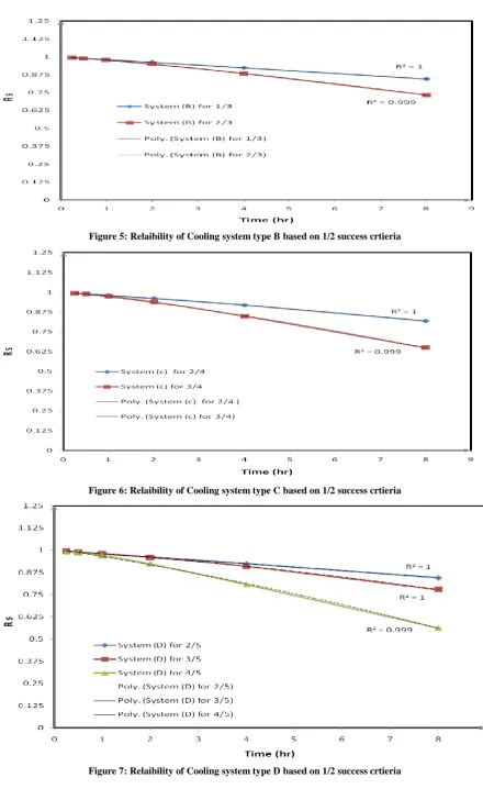
Figure 5: Relaibility of Cooling system type B based on 1/2 success crtieria

Figure 6: Relaibility of Cooling system type C based on 1/2 success crtieria

Figure 8: Cooling System Relaibility versus redundant percentage during steady state condition

Figure 9: Cooling System Relaibility versus redundant percentage during transient condition

1

0.9

0.8

0.7

0.6

0.5

R s

0

25 33 50 100

RD%

0.9

0.85

0.8

0.75

0.7

0.65

0.6

0.55

0.5