389
RELIABLE SHORT TERM LOAD FORECASTING USING
SELF ORGANIZING MAP (SOM) IN DEREGULATED
ELECTRICITY MARKET
1 Z. H. BOHARI, 2 H.S. AZEMY, 3M. N. M. NASIR, 4M. F. BAHAROM, 5M. F. SULAIMA, 6M. H.
JALI
1,2,3,4,5,6
Faculty of Electrical Engineering, Universiti Teknikal Malaysia Melaka (UTeM)
E-mail: [email protected], [email protected]
ABSTRACT
Load demand prediction is important for electric power planning and must be assessed with proper model. The power utility needs to forecasts in order to supply energy to consumer without interference. Neural Networks method is the most popular research topic have been done over the last decade. However, the use of Kohonen Self Organizing Map (SOM) not really explored. This paper present a forecasting method based on type of unsupervised learning neural networks. The main purpose of this project is to investigate the self organizing maps (SOM) neural networks can be used to forecast load demand. In this project, the SOM network is explored to understand the technique of SOM. In addition, this project targeted to improve the accuracy of short term loads forecasting through SOM neural networks technique. This study are focused on testing the first eight hours of the day to be forecast in order to identify its common patterns with the historical database previously trained by neural network. Weekdays data were us as their patterns same. After training, the data were testing and then forecasted. Finally the errors were compared. The MAPE error is 0.322%, 0.128% and 0.64% which is below than 3%. It show that SOM able to use in load forecasting.
KeyWords: Short Term Load Forecasting, Self Organizing Map (SOM), Normalization, Neural Networks.
1. INTRODUCTION
Forecasting is the process of making proclamations about events whose actual outcomes have not yet been observed or can define it as estimates of future value [1]. Load forecasting is an estimation of power demand at some future period. Load forecasting used by Power Utilities Company to predict the amount of power needed to supply the demand. Electric load forecasting has been a major area of research since the last millennium and it is a key to realization for many of the decision makers in the energy division, from power generation to operation of the system [2]. Electric industry wants to predict load demands in the short, medium and long term. Load forecasting can be classified into 3 different types according to the forecast period short-term forecasting, medium-term forecasting and long-term forecasting. Short-term forecasting usually makes forecasts from one hour to one week, medium-term forecasting concerns the future electric load from a week to a month, and long-term forecasting often predicts the load of one year or even longer. Due to research interest and industrial necessities short term load forecasting has gained great attention compared to others. The short-term forecasting is used for guiding and organization
power generation, and also as input to do load-flow studies [3]. Load forecasting has always been important for planning and operational decision conducted by power co. With supply and demand inconsistent and the variety of weather conditions and energy prices growing by a factor of ten or more during peak circumstances, load forecasting is
really major for utilities. Short-term load
390 Therefore development new forecasting model to forecasting electricity load demand which will minimize the error of forecasting is necessary need in Malaysia. The main purpose of this study is to investigate the self organizing maps (SOM) neural networks can be used to forecast load demand.
2. LITERATURE REVIEW
2.1 A Brief Background of Load Forecasting
Short-term load forecasts (STLF) are required for the control and scheduling of power systems [4]. STLF is basically aimed at predicting system load with a leading time of one hour to seven days, which is necessary for adequate scheduling and operation of power systems. STLF traditionally has been an essential component of Energy Management Systems (EMS) as it provides the input data for load flow and contingency analysis [5]. There are a large variety method have been developed for STLF load forecasting techniques grouped broadly in three major groups,
traditional forecasting technique, modified
traditional technique and soft computing technique [6].
Neural networks are currently the most popular method to develop load forecasting tools. Multilayer perceptron (MLP) is the main structure used in these models [4, 5] but other techniques like self-organizing maps [6] or recurrent networks [7] are also good candidates for promising results. Fuzzy logic and other types of artificial intelligence are also present in recent literature especially as part of hybrid methods [8, 9, 10].
2.2 Load Forecasting Using SOM networks
SOM is one type of ANN. SOM acronym is stands for self-organizing maps and it was introduced by T. Kohonen. SOM is a popular neural network based on unsupervised learning, which is not necessary to provide the network with the expected output during the training period. Instead, the network is giving with training data set is usually with the aim of a clustering or classify them. SOM neural networks ability to associate new data with similar learnt data can be applied to forecasting applications [12, 13]. The application of SOM to forecasting can be described in three steps:
1) Training.
• The cells of the map in the top left corner
contain a linear combination of the vectors in the database. It is shown that the content of each cell does not resemble the content of its neighbours. After training, the map in the bottom left corner show how the cells are arranged so that each one is similar to its
neighbours. Also, the whole input space is covered.
2) Association.
• The image in the top centre shows a data
vector. At the time of forecasting, only the known data is used as input to find the cell in the trained map that best matches it.
3) Forecasting.
• The information stored in the best matching
cell is split into the part that was used to match the input and the part that is used to produce a forecast.
3. METHODOLOGIES
Below in Flowchart 1 shows all stages that involved in Short Term forecasting using SOM.
Flowchart 1: SOM Forecasting Stages
3.1 SOM data organization
The previous load demand data is used as input data. The data include daily load demand value in hourly for one month of January in 2009 and 2010 for training and 2011 for testing. Only working days are chosen. Data are divided into 8 main groups by hourly which is [H1, H2, H3, H4, H5, H6, H7, and H8]. H1 to H8 is for first 8 hour of the day. The data consist 8 hour for a day. For training, the input data are labelled as A1 to A43. A1 to A43 is for first 8 hours per day only in weekdays in 2 month. For testing are labelled as B1 to B21. B1 to B21 is for weekdays in a month.
3.2 SOM for training
For training the data structure must be normalized. The normalization is copied to the map structure during the trained SOM. There are 4 types of normalization which is (‘var’, ‘range’, ‘log’, or
‘logistic’). The ‘var’ data input will normalize the
variance variable to unity and the means to zero. For the ‘range’ input data will scale the variable
Step 1 • Data Organization
Step 2 • Data Training
Step 3 • Data Testing
Step 4 • Data Forecasting
391
values between zero and one. The ‘log’ is a
logarithmic transformation and the ‘logistics’ or
softmax transformation scales all possible values between zero and one. The optimum number of neurons must be considered during normalization.
3.3 SOM for testing
After training, the maps are tested with load data on year 2011. This method is to associate the most similar days of 2011 formed by days of 2009 and 2010. This will obtained the pattern for the most suitable day.
3.4 Forecasting load data
After testing, the first 8 hours of the day will be forecast. The curve of load demand forecasting and actual curve is obtained by the software.
3.5 Percentage error calculation
To express the accuracy of the results, the percentage error is calculated using mean absolute
percentage error (MAPE) based on actual load data and forecast load result. The equation of MAPE is:
% 100% (1)
where: = forecasted load; = real load;
= forecasting number
4. RESULTS AND DISCUSSION
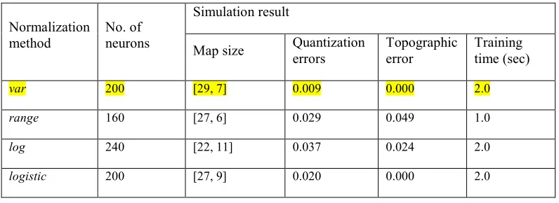
Based on simulation result using SOM, the best result according to the three main criteria (less quantization & topographic error, and lower
training times) is ‘var’ normalization method. The
numbers of neurons used is 200. The quantization
and the topographic errors for ‘var’ are (0.009,
[image:3.612.108.506.351.496.2]0.000) and the training time is (2.0 sec)
Table I: Comparison of Results using Four Normalization Methods
Normalization method
No. of neurons
Simulation result
Map size Quantization
errors
Topographic error
Training time (sec)
var 200 [29, 7] 0.009 0.000 2.0
range 160 [27, 6] 0.029 0.049 1.0
log 240 [22, 11] 0.037 0.024 2.0
[image:4.612.315.528.49.463.2]
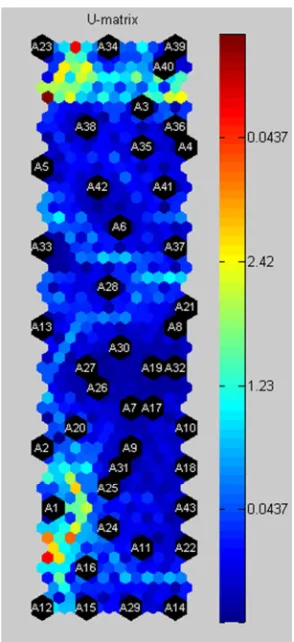
392 Using the best normalization result, U Matrix is mapped to further analyse the forecasting result. In training phase, U Matrix mapped arranged each set of data according to similarity to its neighbours. Figure 1 below shows the trained U Matrix and the day labels assigned to each cell.
Figure 1: Training SOM for year 2009 and 2010
[image:4.612.125.272.169.490.2]After finishing the testing stage, the map show the training data (2009 & 2010) and testing data (2011) are mapping in similar group. Figure 2 below show the testing map assigns the winning cells and these results are then evaluate to do load forecasting.
Figure 2: Testing SOM for year 2009, 2010 and 2011
393 Figure 3: The winner cell consist A19 (1/27/2009) and A32 (1/14/2010), and B4 (1/6/2011) as testing day.
[image:5.612.320.513.283.393.2]Figure 4: The winner cell consist A26 (1/6/2010), A27 (1/7/2010) and A30 (1/12/2010), and B2 (1/4/2011) as testing day.
Figure 5: The winner cell consist A25 (1/5/2010) and A31 (1/13/2010), and B17 (1/25/2011) as testing day.
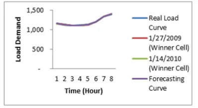
[image:5.612.155.236.315.381.2]Refer to Figure 6, 7, and 8 below show the curve of the both winner cell, real load curve and forecasting curve for first 8 hours. Based on the load demand plot in Figure 6, 7 and 8 for each day, it can be clearly seen that for each day, the load demand seems to share the same pattern. It can clearly see that the graph is gradually increased at hour 6 because during this time the office hours just started.
Figure 6: Curve of winner cell A19 (1/27/2009) and A32 (1/14/2010), real load curve B4 (1/6/2011) and
forecasting curve
Figure 7: Curve of winner cell A26 (1/6/2010), A27 (1/7/2010) and A30 (1/12/2010), real load curve B2
(1/4/2011) and forecasting curve
Figure 8: Curve of winner cell A25 (1/5/2010) and A31 (1/13/2010), real load curve B17 (1/25/2011) and
forecasting curve
[image:5.612.95.294.542.651.2]Daily MAPE errors are shown in Table II. The MAPE errors for each date are 0.322%, 0.128% and 0.64% which indicates the ability of SOM to do forecasting is proven effective. The errors produced from the simulation are less than 3% and again this shown that SOM have the right attributes to do load forecasting.
TABLE II: MAPE error In January
Days MAPE
(%) 1/4/2011 0.322
1/6/2011 0.128
1/25/2011 0.64
The result of the forecast is very good and can be said accurate as the MAPE level are very low (less than 1%) for 3 different dates.
5. CONCLUSION
[image:5.612.356.478.553.627.2]394 easily with the SOM based on the graphical result from the U-matrix. The results of MAPE Error shows a low index error which is below than 3%. It shows that the performance of SOM method gives better result as industry model for short term load forecasting. This paper has developed a model that can improve the accuracy the load forecasting. For the future research, the input variable such as meteorological data can be considered due to the different load pattern.
REFERENCES:
[1] Sergio Valero1, Carolina Senabre1, Miguel López1, Juan Aparicio2, Antonio Gabaldón3
and Mario Ortiz1, “Comparison of Electric
Load Forecasting between Using SOM and
MLP Neural Network”,Journal of Energy and
Power Engineering 6, 2012, pp411-417
[2] Weron, Rafal, “Modeling and Forecasting
Electricity Loads and Prices: A Statistical
Approach”. John Wiley & Sons, Ltd. 2007.
[3] K. Y. Lee, Y. T. Cha, and J. H. Park,
“Short-Term Load Forecasting Using An Artificial
Neural Network,” IEEE Trans. on Power
Systems, vol. 7, Feb. 1992, pp. 124-132 [4] S. J. Kiartzis, A. G. Bakirtzis, V. Petridis, 1995,
“Short-term load forecasting using neural networks” Electric Power Systems Research Volume 33, Issue 1, April 1995, Pages 1-6. [5] M. Sforna, F. Proverbio, 1995, “A neural
network operator oriented short-term and online load forecasting environment”, Electric Power Systems Research Volume 33, Issue 2, May 1995, Pages 139-149.
[6] M. Cottrell, B. Girard, and P. Rousset, “Forecasting of curves using a Kohonen classification,” J. Forecast., vol. 17, 1998, pp. 429–439,
[7] J. Vermaak and E. C. Botha, “Recurrent neural networks for short-term load forecasting,” IEEE Trans. Power Systems, vol. 13, no. 1, 1998, pp. 126–132.
[8] D. Srinivasan, A. C. Liew, and C. S. Chang, “Forecasting daily load curves using a hybrid fuzzy-neural approach,” IEE Proc.—Gener. Transm. Distrib., vol. 141, no. 6, 1994, pp. 561–567.
[9] H. R. Kassaei, A. Keyhani, T.Woung, and M. Rahman, “A hybrid fuzzy, neural network bus load modeling and predication,” IEEE Trans. Power Systems, vol. 14, no. 2, 1999, pp. 718– 724.
[10] M.H. Jali, Z.H. Bohari, M.F. Sulaima, M.N.M. Nasir, H.I. Jaafar, "Classification of EMG Signal Based on Human Percentile using SOM", Research Journal of Applied Sciences, Engineering and Technology, Vol 8 (2), 2014, pp. 235 - 242.
[11] M.H. Jali, I.M. Ibrahim, Z.H. Bohari, M.F. Sulaima, M.N.M. Nasir, ”Classification Of Arm Movement Based On Upper Limb Muscle Signal For Rehabilitation Device”,
Journal of Theoretical and Applied
Information Technology, Vol 68 (1), 2014, pp. 125 – 137.