WAVELET VISIBLE DIFFERENCE MEASUREMENT BASED
ON HUMAN VISUAL SYSTEM CRITERIA FOR IMAGE
QUALITY ASSESSMENT
1NAHID MOHAMMED, 2BAJIT ABDERRAHIM, 3ZYANE ABDELLAH, 4MOHAMED LAHBY
1Asstt Prof., Department of Electrical Engineering, FSTM, Hassan II University, Mohammedia-Casa
2Asstt Prof., Department of Systems Analysis and Design, FSR, Mohamed V University, Rabat
3Asstt Prof., Department of Computer Science and Mathematics, ENSAS, Cadi Ayyad University, Safi
4Asstt Prof., Department of Computer Science, FSTM, Hassan II University, Mohammedia-Casa
E-mail: [email protected], [email protected], [email protected],
ABSTRACT
A reliable quality measure is a much needed tool to determine the type and amount of image distortions. To improve the quality measurement include incorporation of simple models of the human visual system (HVS) and multi-dimensional tool design, it is essential to adapt perceptually based metrics which objectively enable assessment of the visual quality measurement. In response to this need, This paper proposes a new model of image quality measurement called the Modified Wavelet Visible Difference Predictor MWVDP based on various psychovisual models, yielding the objective factor called Probability Score (PS) that correlates well with visual error perception, and demonstrating very good performance. Thus, we avoid the traditional subjective criteria called Mean Opinion Score (MOS), which involves human observers, are inconvenient, time-consuming and influenced by environmental conditions. Widely blurriness or blockiness. Besides the PS score, the model MWVDP provides a map of the visible differences VDM (Visible Difference Map) between the original image and its degraded version. To quantify human judgments based on the mean opinion score (MOS), we measure the covariation between the subjective ratings and the degree of distortion obtained by the probability score PS.
Keywords: JPEG and JPEG2000 Image Compression, Visual Perception, Luminance and Contrast Masking, Mean Opinion Score MOS, Objective and Subjective Quality Measure.
1. INTRODUCTION
Lossy image compression techniques such as JPEG2000 allow high compression rates, but only at the cost of some perceived degradation in image quality. Image quality is ultimately measured by how human observers react to compressed/degraded images and many evaluation methods are based on eliciting ratings of perceived image quality. To compare and evaluate these techniques, we need naturally to measure the visual quality of the images by taking into account the famous factor Mean Opinion Score MOS [3], [12]. A variety of Offered mathematical measures, to estimate the quality of distorted images based on comparisons pixel to pixel, are still used, such as: the Mean Squared Error (MSE) and the Peak Signal to Noise Ratio (PSNR). These measures often deliver a poor correlation versus the factor MOS. However, the
because the distortion introduced on an original image does not have the same effect on the quality of its degraded version. The wavelet transform is one of the most powerful techniques for image compression. Part of the reason for this is its similarities to the multiple channel models of the HVS. In particular, both decompose the image into a number of spatial frequency channels that respond to an explicit spatial location, a limited band of frequencies, and a limited range of orientations. Despite this limitation the quality measure still a goal of the wavelet visible difference predictor WVDP [8] to visually optimize the visual quality performance of the image coding schemes.
Knowing these constraints and exploiting the wavelet decomposition, we have been urged to develop a new wavelet image coding metric based on psychovisual quality properties called, Modified Wavelet Visible Difference Predictor MWVDP based on the WVDP model [A] used to predict visible differences between an original and compressed (noisy) image, and yields a Probability Score PS serving for image quality measure. We also determine the correlation between the PS score and the human judgments based on the mean opinion score (MOS). We compare the test results of different quality assessment models with a large set of subjective ratings gathered for image series which consist of a base image and their compressed versions with JPEG and JPEG2000 coders. All the objective measures which we developed depend on the viewing distance V of the observer towards the perceived image. This paper is structured as follows. In section 2, we present the objective quality metrics. Section 3 details the setup of wavelet perceptual tools for objective metric and probability score computing. Section 4 presents the used experimental methods for subjective quality metric. In section 5 obtained results are presented and discussed. The last section concludes.
2. OBJECTIVE QUALITY METRICS
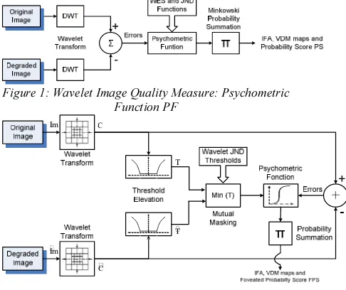
The PF model as shown in figure 1, consists of 1) decomposing the images into a wavelet coefficients [7], 2) performing wavelet detection thresholds, 3) estimating errors for each subband in DWT domain [7], 4) computing the probability summation Minkowski summation [3], [8] based on psychometric function and finally 5) obtaining the PS score, the IFA and VDM maps. Figure 2 shows the component parts of the MWVDP model, which is based on the VDP image quality assessor. It performs respectively wavelet transformation, wavelet detection thresholds, luminance and contrast masking, mutual masking,
[image:2.595.304.547.268.472.2]errors calculation, probability computation based on psychometric function, Minkowski summation, and finally yields probability score PS. The original and the noisy images are first transformed to the DWT domain using a 5 wavelet level decomposition based on the 9/7 Biorthogonal wavelet basis [10]. The differences between the original and noisy images (the wavelet errors) are tested against a wavelet JND threshold to check if the errors are under or bellow this threshold. In other hand, we verify if errors are or not visible.
Figure 1: Wavelet Image Quality Measure: Psychometric Function PF
Im
C
C
T
Im
T
Figure 2: Modified Wavelet Visible Difference Predictor MWVDP model
3. WAVELET PERCEPTUAL TOOLS FOR
OBJECTIVE METRIC
3.1 Quantization Error Sensitivity Function
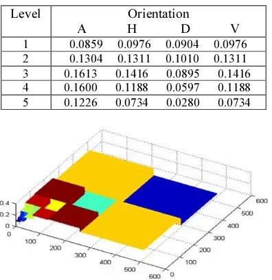
must measure the visibility thresholds for individual basis function and error ensembles. The wavelet coefficients at different subbands and locations supply information of variable perceptual importance to the HVS. In order to develop a good wavelet-based image coding algorithm that considers HVS features, we need to measure the visual importance of the wavelet coefficients. Psychovisual experiments were conducted to measure the visual sensitivity in wavelet decompositions. Noise was added to the wavelet coefficients of a blank image with uniform mid-gray level. After the inverse wavelet transform, the noise threshold in the spatial domain was tested. A model that provided a reasonable fit to the experimental data is done in table 1.
[image:3.595.92.290.405.609.2]As shown in figure 3 (for a viewing distance of 4) error sensitivity increases rapidly with wavelet spatial frequency, and with orientation from low pass frequencies to horizontal/vertical to diagonal orientations. Its reverse form yields the wavelet JND thresholds matrix.
Table 1: Error Contrast Sensitivity in the DWT Domain for V = 4.
Level Orientation
A H D V
1 0.0859 0.0976 0.0904 0.0976 2 0.1304 0.1311 0.1010 0.1311 3 0.1613 0.1416 0.0895 0.1416 4 0.1600 0.1188 0.0597 0.1188 5 0.1226 0.0734 0.0280 0.0734
Figure 3: Wavelet Error Sensitivity Function for V = 4
3.2 Wavelet Perceptual Masking Model Setup
In this work, three visual phenomena are modeled to compute the perceptual weighting model setup matrix: the JND thresholds or just noticeable difference, luminance masking (also known as light adaptation), contrast masking [1], [5] and the contrast sensitivity function CSF [1]. The JND thresholds are thus computed from the base detection threshold for each subband. The mathematical model for the JND threshold is
obtained from the psychophysical experiments adopted by Watson [10] corresponding to the 9/7 biorthogonal wavelet basis. In image coding, the detection thresholds will depend on the mean luminance of the local image region and, therefore, a luminance masking correction factor must be derived and applied to the contrast sensitivity profile to account for this variation. In this work, the luminance masking adjustment is approximated using a power function; here we adopt the model used in JPEG2000 with a factor exponent of 0.649. Another factor that will affect the detection threshold is the contrast masking also known as threshold elevation, which takes into account the fact that the visibility of one image component (the target) changes with the presence of other image components (the masker). Contrast masking measures the variation of the detection threshold of a target signal as a function of the contrast of the masker. The resulting masking sensitivity profiles are referred to as target threshold versus masker contrast functions. In our case, the masker signal is represented by the wavelet coefficients of the input image to be coded while the target signal is represented by the quantization distortion. The strategy of the perceptual model implementation is summarized in the scheme 4 and follows the following stages. First, the original image is decomposed in the DWT domain C(λ,θ,i,j) into 5
decomposition levels λ and in 3 orientations θ corresponding practically to the cortical decomposition of the human visual system HVS. Second, we express the wavelet coefficient ratios against the contrast mean Vmean (128 for 8 bits gray level image), which depends on the image size, to produce the t(λ,θ,i,j) thresholds expression as:
[image:3.595.312.502.547.670.2]and ) , , , (
(
,
,
,
)
mean j i tV
j
i
C
T aθ
λ
θ λ =(1)
)
,
,
,
(
1
)
,
,
,
(
j
i
t
j
i
JND
θ
λ
θ
λ
=
Figure 4: Wavelet Perceptual Masking Algorithm Setup
The JND(λ,θ,i,j) is adjusted by the factor aT
0.649. The luminance masking and contrast masking adjustment are formulated as:
(2) ) , , , ( ). , , , ( ) , , , ( , 1 max ) , , , ( ) , , , ( ) , , , ( ' ' max = = ∈ j i a j i JND j i C j i a and V j i LL C j i a L c a mean L T θ λ θ λ θ λ θ λ λ θ λ ) , , , ( ' '
max LLi j
Cλ : The DWT coefficient, in the LL subband, that spatially corresponds to location(λ,θ,i,j).
/2
/2
, max 5, 0.6' ' max max ∈= = =
= i λ −λ and j j λ −λ λ
i
We alter the amount of masking in each frequency level of the decomposition. This is necessary in the case of the critically sampled wavelet transform to reflect the fact that coefficients at higher levels in the decomposition represent increasingly larger spatial areas and therefore have a reduced masking effect. Typical values for a 5 level decomposition are b(f)=[4 ,2 ,1,0.5 ,0.25] for decomposition
levels 1, 2, 3, 4, 5 respectively. In addition, there is a factor of two difference in the masking effect for positive and negative coefficients, i.e.,
plus
neg b
b =2. . This allows the model to account for
the fact that masking is more reliable on the dark side of edges, i.e., for negative coefficients [8]. The alteration routine, for the original image for example, respects the following law:
. 0 ) , , , ( si ) , , , ( ). ( . 2 (3) , 0 ) , , , ( si ) , , , ( ). ( ) , , , ( < > = j i t j i C f b j i t j i C f b j i alter θ λ θ λ θ λ θ λ θ λ
The threshold elevations T (equation 4) and '
T are
calculated as follows:
(
( , , , ), ( , , , ))
(4) max) , , ,
( i j JND i j alter i j
T λθ = λθ λθ
The mutual masking
m
M is the minimum of the two threshold elevations and respects the following relation:
(
( , , , ), ( , , , ))
(5) min) , , ,
( i j T i j T' i j
Mm λθ = λθ λθ
3.3 Probability Score and Visible Difference Map based on Just Noticeable Difference Thresholds
A psychometric function (equation 6) and its improved version the equation MWVDP (equation 7) are then applied to estimate the error detection
probabilities for each wavelet coefficient and convert these differences, as a ratio of the wavelet JND thresholds, to sub-band detection probabilities. This factor means the ability of detecting a distortion in a subband (λ,θ) at location (i,j) in the DWT field.
(
)
(6)
exp
1
) , , , ( ) , , , ( ) , , , (
−
−
=
β α θ λ θ λ θ λ j i j i PF j iJND
D
Pb
(
)
(7)
exp
1
) , , , ( ) , , , ( ) , , , (
−
−
=
β α θ λ θ λ θ λ j i m j i MWVDP j iM
D
Pb
WhereD(λ,θ,i,j)=C(λ,θ,i,j)−C'(λ,θ,i,j). The parameters β (between 2 and 4) and λ (between 1 and 1.5) for each metric is chosen to maximize the correspondence of the DWT probability error
XXX j i Pb ) , , ,
(λθ , to optimize the probability summation
[A], [A] and especially to maximize the correlation between the objective metrics and the observers note MOS.
The output of the models PF and MWVDP is a probability map, i.e., the detection probability at each pixel in the image. Therefore, the probability of detection in each of the sub-bands (channels) must be combined for every spatial location in the image. This is done using a product series [4], [6].
(
1 ( , ,, ))
(8) 1 ) , , , ( = −∏
− b bd i j P i j
P λθ λθ
Finally, to confirm the subjective quality ordering of the images we also defined a simple score PS (varie between 0 and 1 included) for the M X N image size as:
(9) ) , , , ( . 1 , ,
∑
= N M j id i j
P N M
PS λθ
Figure 5(a): Original Image Threshold Elevation
Figure 5(b): Mutual Masking
Figure 5(c): Just Noticeable Differences JND
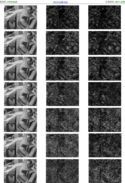
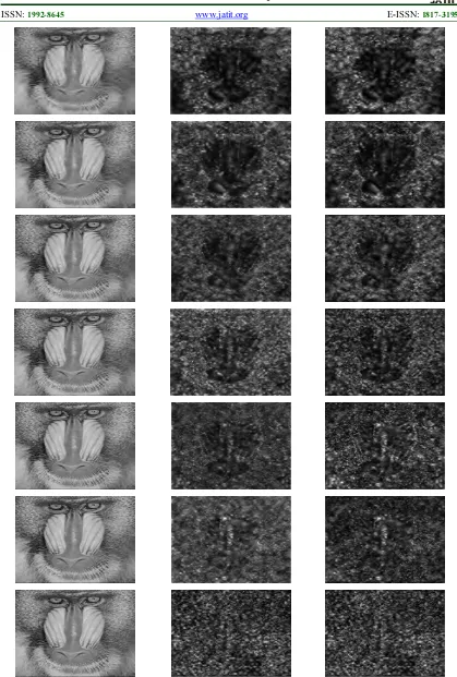
[image:5.595.90.278.103.253.2]Figure 5(d): VDM Map Errors
Figure 5: Threshold Elevation, Mutual Masking, JND Thresholds and VDM Errors for 'Barbara’ Image at V=4
4. SUBJECTIVE QUALITY METRIC
4.1 Conditions of Subjective Quality Evaluation
[image:5.595.99.508.120.756.2]The subjective quality evaluation is normalized by the recommendations of the CCIR [11], [13]. However, these recommendations are designed, originally, for the television image without taking into account the measure of the degradations with the original image. Our purpose is to measure the distortions between two images instead of the quality of a single image by adopting the tests of comparative measures: We suppose furthermore that the images can be edited, zoomed and observed at the lowest possible distance. Therefore, we refer to the conditions of evaluation which were used by Fränti where the recommendations of the CCIR are partially respected in table 2. The room of evaluation is normalized in order to make tests without introducing errors relative to the study environment. All the light sources, other than those used for the lighting of the room are avoided because they degrade significantly the image quality. The screen is positioned so that no light source as, a lamp or a window, affects directly the observer's vision field, or causes reflections on the some surfaces on the screen. The subjective measure serves only, in our study, to estimate the objective measures in terms of the coefficient of correlation which will be described in the following paragraph.
Table 2: Conditions of Subjective Quality Evaluation
Image Quality Photographic Images
Observation Conditions
Environment of Normal Desk
Viewing Distance V In the free Appreciation of the Observer
Observation Duration Unlimited
Number of Observers Between 15 and 39
[image:5.595.97.284.286.561.2] [image:5.595.100.514.482.721.2]4.2 The Objective Measure Correlation Coefficients
To determine the objective measure correlation (noted by the vector X) with the subjective measure (noted by the observation vector Y), we use the correlation coefficient which is defined by the following equation:
(
)
(
)(
)
(
)
(
)
(10)
,
2 n 1 2 n 1 n 1∑
∑
∑
= = =−
−
−
−
=
i i i i i i iY
Y
X
X
Y
Y
X
X
Y
X
ρ
Where Xi andYi, i=1 to n, are, respectively, the components of vectors X and Y. n represents the number of values used in the measure. X and Y
represent, respectively, values average of vectors X and Y, given according to the following formula:
(11)
1
1∑
==
n n iX
n
X
We agree to associate the variance value determined by the relation 12 with every MOS average.
(
)
(12)
1
)
(
1 2∑
=−
=
n i iX
X
n
X
Var
5. EXPERIMENTAL RESULTS AND
DISCUSSION
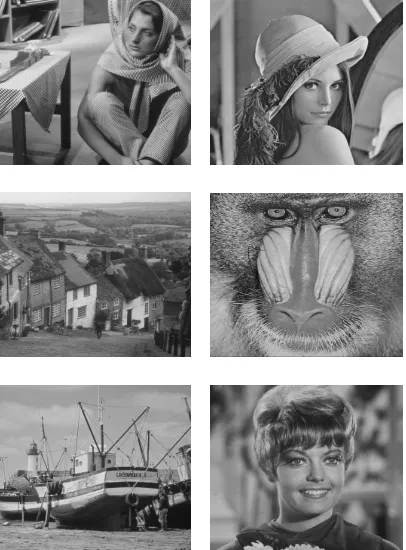
The test images are shown on a screen CRT of PC, with 10.5 cm x 10.5 cm (512x512 pixels images) [11], [12]. The MOS scale extends from 0 to 10 (2: very annoying degradation, 4: annoying, 6: a little bit annoying, 8: perceptible, but not annoying, 10: Imperceptible). We also tuned the possibility to the observers to give notes by half-values. To calculate the final subjective measure of a degraded image, we determine the average of notes given by the observers. If the correlation is used through a single type of image, n will take the value 10 or 8 (JPEG or JPEG2000, 512x512 coded images). If the correlation is used through all the types of image, n will take the value of the total number of images (60 for the JPEG 512x512 coded images and 48 for those JPEG2000 512x512 coded images). Figure 6 presents examples of test images database.
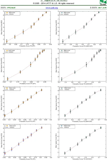
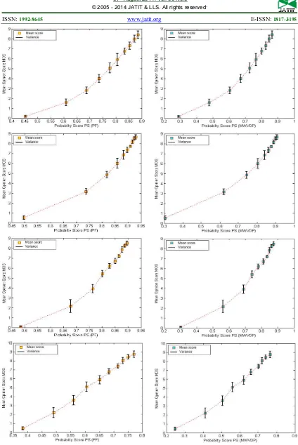
In figures 7and 8 we plot the MOS subjective measures vs the PS objective measures for the test images, compressed JPEG and JPEG2000. Let observe that the evolution of the PS factors is quasi-linear according to that of the MOS observer notes. What proves a better correlation between both measures.
Figures 9 and 10 show the IFA maps given by PF and MWVDP models for JPEG2000 compressed images at 0.05, 0.1, 0.2, 0.3, 0.4, 0.5 and 0.75 bpp. Notice that IFA maps follow the image nature, and represent faithfully the visible error structures. Generally, both metrics predict more or less the same perceived quality evaluation.
Finally, the measures of the correlation coefficients are given in table 3. The correlation coefficients reach 0.8343 and 0.9162 through all images coded JPEG2000; and reach 0.8672 and 0.9198 through all images coded JPEG; respectively by the PF and MWVDP metrics. They reach 0.8520 and 0.8964 through all images for two types of coders. The MWVDP model proves its superiority in the correlation towards its corollary PF.
[image:6.595.306.509.425.700.2]
6. CONCLUSION
We have demonstrated the superiority of the MWVDP model by proving its best correlation with the MOS in consideration to other models commonly used for evaluating the image perceived distortions. Indeed, the MWVDP model has a number of advantages. It provides maps of errors spatial IFA (Image Fidelity Assessor) and VDM (Visible Difference Map) in the wavelet domain. It's able to process all these measures by taking into account the observation distance. In addition, it proved its efficiency to process the images degraded with different types of distortions, like, impulsive salt-pepper noise, additive Gaussian noise, blurring images.
REFRENCES:
[1] S. Daly, “Subroutine for the Generation of a Two Dimensional Human Visual Contrast Sensitivity Function”, 233203Y, Technical Report, Eastman Kodak, 1987.
[2] Z. Wang, A. C. Bovik, and L. Lu, “Why is Image Quality Assessment so Difficult”, IEEE International Conference on Acoustics, Speech, and Signal Processing, Vol. 4, 2002.
[3] Z. Wang, A. C. Bovik, H. R. Sheikh, and E. P. Simoncelli, “Image Quality Assessment: From Error Visibility to Structural Similarity”, IEEE Transactions on Image Processing, Vol. 13, N°4, April 2004.
[4] H.R. Sheikh, A. C. Bovik, and G. de Veciana, “A Visual Information Fidelity Measure for Image Quality Assessment”, IEEE Transactions on Image Processing, vol.14, N°.12, Dec. 2005, pp. 2117- 2128.
[5] A. B. Watson, G. Y. Yang, J. A. Solomon, and J. Villasenor, “Visual Thresholds for Wavelet Quantization Error”, Proc. SPIE, 1997, pp. 382-392.
[6] S. J. Daly, “Visible Differences Predictor: An Algorithm for the Assessment of Image Fidelity”, SPIE Proceedings Vol. 1666: Human Vision, Visual Processing, and Digital Display III, 27 August 1992.
[7] S. Mallat., “A Wavelet Tour of Signal Processing”, Third Edition December 25, 2008. [8] A. P. Bradley, “A Wavelet Visible Difference
Predictor”, IEEE Transactions on Image Processing, Vol. 8, N°. 5, 1999.
[9] J. Lubin, “A Visual Discrimination Model for Imaging System Design and Evaluation, Vision models for Target Detection and Recognition”, E. Peli, World scientific, 1995.
[10] Z. Liu, L. J. Karam, A. B. Watson, “JPEG2000 Encoding with Perceptual Distortion Control’’, Inter. Conference on Image Processing, 2003. [11] M. A. Saad and A. C. Bovik, ’’BLIINDS
Code’’, 2012. [Online]. Available: http://live.ece.utexas.edu/research/quality/
[12] R. Soundararajan and A. C. Bovik, “RRED indices: Reduced Reference Entropic Differencing for Image Quality Assessment”, IEEE Trans. Image Process., vol. 21, N°. 2, pp. 517–526, Feb. 2011.
Table 3: Correlation Coefficients between the PS Objective Measures and the Subjective Measures vs the MOS Score of 108 Compressed Images at Viewing Distance V = 4. 24 Observers.
Correlation Coefficients of 8 JPEG2000 Compressed Image Versions
Barbara Lena Goldhill Mandrill Boat Zelda 48 Images
PF 0.9913 0.9885 0.9894 0.9991 0.9917 0.9865 0.8343
MWVDP 0.9954 0.9889 0.9871 0.9984 0.9927 0.9803 0.9162
Correlation Coefficients of 10 JPEG Compressed Image Versions
Barbara Lena Goldhill Mandrill Boat Zelda 60 Images
PF 0.9696 0.9631 0.9668 0.9965 0.9522 0.9624 0.8672
MWVDP 0.9696 0.9699 0.9688 0.9919 0.9518 0.9636 0.9198
Correlation Coefficients of 18 Compressed Image Versions: 8 JPEG2000 + 10 JPEG Compressed Images
Barbara Lena Goldhill Mandrill Boat Zelda 108 Images
PF 0.9777 0.9658 0.9656 0.9826 0.8864 0.8506 0.8520
[image:11.595.88.507.109.722.2]
[image:12.595.87.506.102.723.2]