A PROFICIENT LOW COMPLEXITY ALGORITHM FOR PREEMINENT TASK SCHEDULING INTENDED FOR HETEROGENEOUS ENVIRONMENT

DIFFERENTIAL EVOLUTION AND GENETIC ALGORITHM

BASED FEATURE SUBSET SELECTION FOR RECOGNITION

OF RIVER ICE TYPES

1_{BHARATHI P. T,} 2_{Dr. P. SUBASHINI}

1, 2

Department Of Computer Science, Avinashilingam Institute For Home Science And Higher Education For Women, Coimbatore, India

E-mail: [email protected], [email protected]

ABSTRACT

One of the essential motivations for feature selection is to defeat the curse of dimensionality problem. Feature selection optimization is nothing but generating best feature subset with maximum relevance, which improves the result of classification accuracy in pattern recognition. In this research work, Differential Evolution and Genetic Algorithm, the two population based feature selection methods are compared. First, this paper presents Differential Evolution float number optimizer in the combinatorial optimization problem of feature selection. In order to build the solution generated by the Differential Evolution float-optimizer suitable for feature selection, roulette wheel structure is constructed and supplied with the probabilities of features distribution. To generate the most promising feature set during iterations these probabilities are constructed. Second, Genetic Algorithm minimizes the Joint Conditional Entropy between the input and output variables. Practical results indicate Differential Evolution feature selection method with ten features achieves 93% accuracy when compared with Genetic Algorithm method.

Keywords:Differential Evolution, Genetic Algorithm, Feature Extraction, Confusion Matrix, Probabilistic Neural Network Classifier.

1. INTRODUCTION

One of the most important and crucial tasks in any pattern recognition system is to overcome the curse of dimensionality problem, which forms an inspiration for using a suitable feature selection method. Feature selection also known as feature subset selection, is a problem that has to be addressed in many areas like image recognition, text categorization, bioinformatics, clustering, artificial intelligence and pattern recognition. The reasons behind using feature selection methods include: dimensionality reduction, removing irrelevant and redundant features, reducing the amount of data required for learning, improving methods in accuracy prediction. This has led to the development of a variety of techniques for selecting an optimal subset of features from a larger set of possible features.

The original feature set can be formed by concatenating the features formed by different feature extraction methods. Feature selection consists of choosing, the subset of features among the input features that has maximum prediction power for the output. More formally, let us consider X = (X1,…,Xd) a random input vector and Y a continuous random output variable that has to be

predicted from X. The duty of feature selection consists in finding the features Xi that are most relevant to predict the value of Y.

procedures like ACO, GA, and PSO, is the focus of research in recent years.

The present work is organized as follows: Section 2 describes feature subset selection method. Section 3 describes implementation and experimental results obtained with feature subset selection method. Finally, section 4 concludes with some final remarks and all the references been made for completion of this work.

2. FEATURE SUBSET SELECTION

METHODS

2.1 Differential Evolution

Differential evolution (DE) is a simple optimization method that has parallel, direct search, easy to use, good convergence, and fast implementation properties. The first step in the DE optimization method is to generate a population of NP members each of D-dimensional real-valued parameters, where NP is the population size, and D represents the number of parameters to be optimized. The crucial idea behind DE is a new scheme for generating trial parameter vectors by adding the weighted difference vector between two population members xr1 and xr2 to a third member xr0. The following equation shows how to merge three different randomly selected vectors to create a mutant vector,

V

_ig

,

from the current generation g:

(

jr g jr g

)

g r j g i

j

x

F

x

x

v

, 2 , , 1 , , 0 , ,

,

=

+

×

−

(1)

where

_F

_∈

( )

0

,

1

is a scale factor that control the rate at which the population evolve. The index g indicates the generation to which a vector belongs. In adding up, each vector is assigned a population index, i, which runs from 0 to

NP

−

1

. Parameters

in vectors are indexed with j, which operates from 0 to

D

−

₁

. In addition, DE employs uniform

crossover, also known as discrete recombination, in order to build testing vectors out of parameter values that have been copied from two different vectors. DE crosses each vector with a mutant vector, as specified in Eq. (2):









≤

=

otherwise

x

or

C

rand

if

v

u

g i j r g i j g i j , , , , , ,

)

1

,

0

(

(2)

where

u

j,i,g is the j

th

dimension from the ith trial vector along the current population g. The crossover probability

_∈

[ ]

0

,

1

r

C

_{, is a user defined}

value that controls the fraction of parameter values that are copied from the mutant [8, 11].

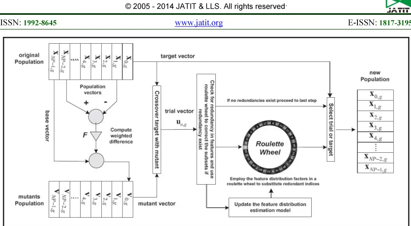
In order to utilize the float number optimizer of DE in feature selection, a number of modifications have been suggested by Rami N. Khushaba. Fig. 1 is taken from [Ref 7], shows the block diagram of the DEFS method. Like all population-based optimizers the DEFS attacks the starting point problem by sampling the objective function at multiple, randomly chosen initial points, referred in Fig. 1 as original population. Thus an original population matrix of size

(

NP

_×

DNF

)

containing NP randomly chosen initial vectors, xi, i = {0, 1, 2, . . . ,

NP

₋

₁

_{} is created, where DNF is}

the desired number of features to be selected. In the DEFS method, the search space is limited between 1 and the total number of features (NF). The next step in the method is to generate a set of new vectors from the original population, referred in Fig. 1 as mutant population, in which each vector is indexed with a number from 0 to

NP

−

1

[7].

For each position in the original population matrix, a mutant vector is formed by adding the scaled difference between two randomly selected population members to a third vector, according to Eq. (1). Unlike the original DE that uses a constant scale factor, the DEFS allows the scale factor to change dynamically as follows:

(

x

jr g

x

jr g

)

rand

C

F

, 2 , , 1 , 1

,

max

×

=

(3)

where c1 is a constant smaller than 1. The effect of this is to allow the population members to oscillate within bounds without crossing the optimal solutions and thereby aiding them to find improved points in the optimal region. Additionally, a system constant with stipulation is implemented as









<

>

=

1

1

,,

, , , , g i j g i j g i j

x

if

NF

x

if

NF

x

(4)

Due to the fact that a real number optimizer is being used, nothing will prevent two dimensions from settling at the same feature indexes. As an example, if the resultant vector is: [3.7353, 20.1000, 13.0000, 4.0000, 13.1471, 10.8478, 20.0000, 21.9286, 15.0000, 8.0789], after rounding the values, the resultant vector values will be [4, 20, 13, 4, 13, 11, 20, 22, 15, 9]. The feature index 4 occurs twice which is completely unacceptable in feature selection method. In order to overcome such a problem, a roulette wheel weighting scheme is utilized [12]. In this scheme, a cost weighting is implemented in which the probabilities of each feature are calculated from the distribution factors associated with it. The distribution factor of feature

f

_j within

the current generation g, is referred as

_FD

_jg

,

which is calculated using below equation:

(

)

(

)

       + + − × − +         + × = j j j j j j j g j ND PD ND PD NF DNF NF ND PD PD a FD max 1 1

, (5)

where PDj is the number of times that feature

j

f

has been used in the good subsets. NDj is the

number of times that feature

f

_j has been used in the less competitive subsets. NF is the total number of features,

a

₁is a suitably chosen positive constant

that reflects the importance of features in PD, and DNF is the desired number of features to be selected. Divide the estimated distribution factors for the current and the next iterations by the maximum value, i.e.,

_FD

_g

₌

_FD

_g

max

(

_FD

_g

)

and _{1 1}

max

(

₁

)

+ +

+

=

g g

g

FD

FD

FD

. Compute

the relative difference according to the following equation:

(

FD

g

FD

g

)

FD

g

FD

g

T

=

+1

−

×

+1

+

(6)

The above equation provides higher weights to features that make obvious improvement in the current iteration in comparison to the previous one. Next add some sort of randomness in this process to avoid selecting the same features every time, to emphasize the importance of unseen features

(

NF

) (

T

)

rand

T

T

₌

₋

₀

_.

₅

_×

₁

_,

_×

₁

₋

₍₇₎

For the remaining iterations, the distribution factors are updated within each iteration as FDg = FDg+1, and FDg+1 hold recently computed values in each iteration.

2.2 Information theory and Genetic Algorithm

2.2.1 Discrete joint conditional entropy (JCE)

This section presents a brief general idea of some concepts of information theory, will be useful to explain the method. In particular, JCE which enables the evaluation of the amount of information that lacks to determine the target output variable [13]. The method anticipated in this paper considers discrete variables. Hence, every continuous variable is discretized by sub-dividing its selection into a finite set of interval. A mean value for each interval is considered respectively.

The conditional entropy of the scalar discrete random variable Y, assuming the event X = xk, is given by:

∑

=

⋅

−

=

N i k i k i

k

P

y

x

P

y

x

x

Y

H

1

)

|

(

))

|

(

log(

)

|

(

(8)

where

P

(

y

_i

|

x

_k

)

is the probability that Y = yi assuming event X = xk. The conditional entropy of Y, considering the knowledge of X, is given by

∑

=

⋅

=

N k k

k

P

x

x

Y

H

X

Y

H

1

)

(

))

|

(

)

|

(

(9)

which define the ambiguity about Y when all the trials of X are known with the following equation below:

)

(

)

,

(

)

|

(

_Y

_X

_H

_X

_Y

_H

_X

H

=

−

(10)

where H(X, Y) is the joint entropy:

∑∑

= =

⋅

−

=

N i N k k i k

i

y

P

x

y

x

p

Y

X

H

1 1

)

,

(

)

,

(

log(

)

,

(

(11)

The concept of joint entropy Eq. (11) can be extended to the following general formulation Eq. (12), where n input variables X1, . . . ,Xn, and N discrete possible values (bins) for each variable are assumed:

)

,...,

,

(

))

,...,

,

(

log(

...

)

,...,

,

(

, , 1

1 1 1

, , 1 1 1 1 1 n n

n i i ni

N i N i N i i n i i n

x

x

y

P

x

x

y

P

X

X

Y

H

∑∑ ∑

= = =

⋅

−

=

(12) where j i j

x

, is event ij of variable Xj, for ij = 1, . . .

,N, and j = 1,. . . ,n. This work defines

)

,...,

(

)

,

,...,

(

))

,...,

(

|

(

1 1 1 n n n

X

X

H

Y

X

X

H

X

X

Y

H

−

=

(13)

2.2.2 Cross entropy function

The cross correlation function is based on a linear adjustment among the variables. For this reason, the method encounters some problems when applied to non-linear systems. The problem of cross correlation function is overcome by cross entropy function (XEF), which is a suitable analysis that is more appropriate for non-linear dynamic relationships.

Normalized mutual information, R, between two signals, X and Y is given below:

)

(

)

|

(

)

(

Y

H

X

Y

H

Y

H

R

=

−

(14)

Parameter R is restricted to [0, 1] interval and represents the amount of information about the target variable that is revealed by the input variable. If X contains all the necessary information to predict Y, then H(Y|X) = 0 and R = 1. If X does not contain information about Y, then H(Y|X) = H(Y) and R = 0.

In this approach the JCE Eq. (13) is directly used as the fitness function of the GA and the objective of the optimization problem is to obtain the input signals X1, . . . ,Xn that achieve the minimum JCE, with the equation below:

))

,...,

(

|

(

min

1

..

1

n X

X n

H

Y

X

X

(15)

More specifically, the goal is to find the optimal input variables. In GA, the chromosomes are composed of all the input variables. The input vector is spread as a first individual in the initial population with the aim of accelerating the convergence of the algorithm. Next, the remaining individuals of the initial population are randomly generated with uniform distribution and standard deviation (

δ

_{) around the seeded individual. The}

GA applied in this work operates on the decimal basis. The chosen crossover genetic operator was the

BLX

₋

α

_{, defined by}

))

(

)

1

(

)

(

(

)

1

(

k

round

g

₁

k

g

₂

k

g

n n n

c

+

=

α

⋅

+

−

α

(16)

where k is the generation;

α

_∈

[

0

,

1

]

with uniform

distribution; n c

g

is the gene n of the child

chromosome c, and n

g

₁ and

g

₂n are genes corresponding to position n of parent chromosome vectors.

After fitness evaluation, the algorithm organizes the individuals by their fitness ranking the indexes of the individual vectors from best to worst on there performance. Next, the crossover operator is implemented in order to create a new

generation. Each individual has a probability of reproduction that is given by its fitness value. More adapted individuals (i.e. the individuals in higher positions of the ranking) have more probability of participating in the crossover operation.

The selection process based on a uniform random variable is not adequate; hence random variable is used to select individuals to participate in the crossover. Crossover must have probability density is larger for small value than large values in favor of individuals. To carry out this, random variable

σ

'is used:

1

1

'

−

−

=

_a

a

e

e

σ

σ

₍₁₇₎

where a is a positive constant, and

σ

_∈

[

0

,

1

]

is a

random variable with uniform distribution. This procedure makes it feasible to increase or decrease the selective search. Search space is increased for faster convergence. The algorithm may constrain the population to a local minimum for larger search space. According to discrete random variable individuals are selected for crossover by the rank i,

)

(

_T

_σ

'

round

i

₌

₍₁₈₎

where T, total number of individuals.

2.3 Probabilistic Neural Networks Classifier

Probabilistic Neural Networks (PNN) is a widely used classification. The inbuilt advantage of the PNN architecture is the speed with which it can be trained and can handle data that has points outside the norm thus performing better than other neural architectures. PNN classifier is used to classify unknown feature vectors into predefined classes, where the Probability Density Function (PDF) of each class is estimated by kernel functions [9]. The general form of the PDF estimator is given by

∑

=

−

n

k

k

x

x

w

n

1

)

(

1

σ

σ

(19)

where, x = unknown (input), xk = kth sample, w = weighting function, σ = smoothing parameter.

2.4 Confusion Matrix

of 9 samples for each 5 classes. The entries have the following meanings, True negative (TN) is the number of correct negative predictions, False Positive (FP) is the number of incorrect positive predictions, False Negative (FN) is the number of incorrect negative predictions, True Positive (TP) is the number of correct positive predictions.

Precision, Sensitivity and specificity the performance metrics for a classification function. Sensitivity measures the percentage of actual positives which are correctly identified. Specificity measures the percentage of negatives which are correctly identified. Precision is the percentage of the predicted positive cases that were correctly identified [14, 16].

Precision is the fraction of retrieved instances that are relevant

FP

TP

TP

ecision

+

=

Pr

(20)

Sensitivity relates to the test's ability to identify positive results.

FN

of

Number

TP

of

Number

TP

of

Number

y

Sensitivit

+

=

(21)

Specificity relates to the test's ability to identify negative results.

FP

of

Number

TN

of

Number

TN

of

Number

y

Specificit

+

=

(22)

3.IMPLEMENTATION&EXPERIMENTAL

RESULTS

3.1 Image Dataset and Experimental setup

In this research, image dataset consists of different stages of ice formation on river or lake during winter season is considered. Each ice image has a resolution of 3968 x 2976 pixels. This dataset is chosen since it contains various types of ice such as water, snow ice, Boarder ice, and Sheet ice, Frazil Ice/Thin Ice, Juxtaposed Ice/Medium Ice and Consolidated Ice/Thick Ice. The experiments are implemented in MATLAB. These techniques are experimented on 240 different types of ice images with various ice conditions.

3.2 Experimental Results

The features are extracted from first order statistics; second order statistics such as gray level co-occurrence matrix (GLCM) and gray level run length matrix (GLRLM) method. Five features are extracted from first order statistics; they are Mean, Variance, Standard Deviation, Skewness, and

Kurtosis. Inverse Difference Moment, Contrast, Correlation, Energy, Entropy, Homogeneity, Sum Average, Sum Variance, Sum Entropy, Difference Variance, and Difference Entropy are eleven features extracted from GLCM. Short run emphasis, Long run emphasis, Gray Level Uniformity, Run Percentage, Run Length Non-Uniformity, Low Gray Level Run Emphasis and High Gray Level Run Emphasis are the seven features extracted from GLRLM method. Total of 23 features are formed by combining all the features from first order statistics, GLCM and GLRLM methods. The feature set acts as the input for population based feature selection methods [10].

Population based feature selection methods worked out here require the desired number of features (DNF), or the size of feature subsets, to be specified by the user. NF refers to the total number of features in the feature set, then it is understood that

DNF

_≤

NF

_{. For all feature}

selection experiments described in this paper uses a population size of 50, while the stopping criterion is defined as reaching the maximum number of iterations, which was set to 100. Although the methods started from the same initial population, the continuous exploration ability of the DEFS that is aided by the statistical measure, proved to be very useful in searching the feature subspace.

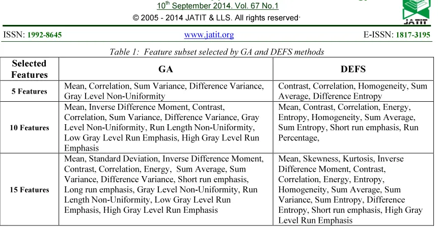
Among the 23 features, the best five, ten and fifteen features selected by GA and DEFS methods are shown in Table 1 and the confusion matrix of TP, TN, FP and FN is shown in table 2 for five, ten and fifteen feature subsets respectively. GA selected feature subset is evaluated by using PNN classifier and the results are shown in Fig 3, and also the performance of GA through PNN classifier is evaluated by performance metrics such as precision, sensitivity and specificity which is shown in Table 3. From Table 3 it is found that the performance of GA is not very competitive when selecting large number of features. This could be related to the cross-over and mutation operators, as they may fail to lead the search for the best large subset toward the global minima when dealing with huge datasets. However, as the number of selected features increases, the performance of GA does not produce good result.

roulette wheel. Accordingly, there is a sort of continuous exploration and exploitation capability associated with the DEFS search procedure. Also, because of the probability is being updated with every iteration, this process will give the DEFS a better capability of finding the features that constitute the best subsets. DEFS selected feature subset is evaluated by using PNN classifier and the results are shown in Fig 3, and also the performance of DEFS through PNN classifier is evaluated by performance metrics such as precision, sensitivity and specificity which is shown in Table 4.

From Table 3, Table 4 and Fig 3, it is found that performance of DEFS method proved to be better than GA method on all images used in the dataset. Thus all the results proved the effectiveness of the DEFS method in searching for the best subsets with 93% accuracy with ten features.

4.CONCLUSION

This research work aims on feature selection methods to measure the effectiveness of machine learning techniques for classification accuracy. The dataset consists of 240 images with different types of ice formation during winter season on River/Lake with five target classes. Population based feature selection methods such as GA and DEFS are experimented in this work. The results obtained by these methods indicate the potential advantages of using feature selection techniques to improve the classification accuracy with less number of feature subset. The limitations of GA, need to handle too many parameters to achieve good performance and it shows lower accuracy rate as the number of feature subset increases. From the result, one can conclude that the performance of DEFS is superior to GA method. DEFS method achieves 93% accuracy when compared with GA method.

REFRENCES:

[1]Isabelle Guyon and Andre Elisseeff, “An Introduction to Variable and Feature Selection”, Journal of Machine Learning Research 3, Pg. No.1157-1182, 2003

[2]L.Ladha and T.Deepa, “Feature Selection Methods and Algorithms”, International Journal on Computer Science and Engineering (IJCSE), Pg. No. 1787-1797Vol. 3 No. 5 May 2011.

[3]Ludwig Jr and et al, “Applications of information theory, genetic algorithms, and neural

models to predict oil flow”, Commun Nonlinear Sci Numer Simulat 14, Pg. No. 2870–2885, 2009.

[4]Yi-Leh Wu and et. al, “Feature selection using genetic algorithm and cluster validation”, Expert Systems with Applications 38, Pg. No. 2727– 2732, 2011.

[5]Bir Bhanu and Yingqiang Lin, “Genetic algorithm based feature selection for target detection in SAR images”, Image and Vision Computing 21, Pg. No. 591–608, 2003

[6]Mingyuan Zhao and et. al.,” Feature selection and parameter optimization for support vector machines: A new approach based on genetic algorithm with feature chromosomes”, Expert Systems with Applications 38, Pg. No. 5197– 5204, 2011.

[7]Rami N. Khushaba and et. al., “Feature subset selection using differential evolution and a statistical repair mechanism”, Expert Systems with Applications 38, Pg. No. 11515–11526, 2011

[8]Ahmed Al-Ani and et. al., “Feature subset selection using differential evolution and a wheel based search strategy”, Swarm and Evolutionary Computation 9, Pg. No.15–26, 2013.

[9]Bharathi P.T and Dr. P. Subashini, “Texture Based Color Segmentation for Infrared River Ice Images using K-Means Clustering”, International Conference on Signal Processing, Image Processing and Pattern Recognition (ICSIPR), 978-1-4673-4862-1/13/$31.00, IEEE Trans, 2013.

[10]Bharathi P. T and P. Subashini, “Texture Feature Extraction of Infrared River Ice Images using Second-Order Spatial Statistics”, International Conference on Computer Vision, Image and Signal Processing, Barcelona, Spain, Proceedings of World Academy of Science, Engineering and Technology 74, Pg. No. 747 – 757, 2013.

[11]Utpal Kumar Sikdar et al.,” Differential Evolution based Feature Selection and Classifier Ensemble for Named Entity Recognition”,

Proceedings of COLING 2012: Technical Papers, pages 2475–2490, COLING 2012, Mumbai, December 2012.

[12]Haupt, R. L and Haupt, S. E, Practical genetic algorithms, 2nd edition, A John Wiley & Sons, Inc., Publication 2004.

[14]Sofia Visa et al., “Confusion Matrix-based Feature Selection”, http://ceur-ws.org/Vol-710/paper37.pdf

[15]http://en.wikipedia.org/wiki/Confusion_matrix

[image:8.595.85.515.81.305.2]

Table 1: Feature subset selected by GA and DEFS methods

Selected

Features GA DEFS

5 Features Mean, Correlation, Sum Variance, Difference Variance, Gray Level Non-Uniformity

Contrast, Correlation, Homogeneity, Sum Average, Difference Entropy

10 Features

Mean, Inverse Difference Moment, Contrast,

Correlation, Sum Variance, Difference Variance, Gray Level Non-Uniformity, Run Length Non-Uniformity, Low Gray Level Run Emphasis, High Gray Level Run Emphasis

Mean, Contrast, Correlation, Energy, Entropy, Homogeneity, Sum Average, Sum Entropy, Short run emphasis, Run Percentage,

15 Features

Mean, Standard Deviation, Inverse Difference Moment, Contrast, Correlation, Energy, Sum Average, Sum Variance, Difference Variance, Short run emphasis, Long run emphasis, Gray Level Non-Uniformity, Run Length Non-Uniformity, Low Gray Level Run Emphasis, High Gray Level Run Emphasis

[image:8.595.84.514.340.442.2]

Mean, Skewness, Kurtosis, Inverse Difference Moment, Contrast, Correlation, Energy, Entropy, Homogeneity, Sum Average, Sum Variance, Sum Entropy, Difference Entropy, Short run emphasis, High Gray Level Run Emphasis

Table 3: Performance metrics of GA through PNN classifier

Method Genetic Algorithm

Feature Subset 5 Features 10 Features 15 Features Classes 1 2 3 4 5 1 2 3 4 5 1 2 3 4 5

Precision 0.5 0.5 0.78 0.39 1 0.67 0.4 0.36 0.58 0 0.33 0.4 0.11 0.43 0.33

Sensitivity 0.44 0.22 0.78 0.78 0.67 0.22 0.67 0.56 0.78 0 0.44 0.22 0.11 0.33 0.44

Specificity 0.89 0.94 0.94 0.69 1 0.97 0.75 0.75 0.86 0.97 0.78 0.92 0.78 0.89 0.78

Classification

accuracy in % 58 44 31

Table 4: Performance metrics of DEFS through PNN classifier Method Differential Evolutation

Feature Subset 5 Features 10 Features 15 Features

Classes 1 2 3 4 5 1 2 3 4 5 1 2 3 4 5

Precision 0.82 0.82 0.78 0.86 0.86 1 0.9 0.89 0.89 1 0.47 0.56 0.63 0.75 0.8

Sensitivity 1 1 0.78 0.67 0.67 1 1 0.89 0.89 0.89 0.78 0.56 0.56 0.67 0.44

Specificity 0.94 0.94 0.94 0.97 0.97 1 0.97 0.97 0.97 1 0.78 0.89 0.92 0.94 0.97

Classification

accuracy in % 82 93 60

Table 5: Confusion Matrix for five-class classification problem Predicted class j by classifier True class i 1 2 3 4 5

Actual classes

Figure1: Block Diagram Of Differential Evolution Feature Selection Method.

0 10 20 30 40 50 60 70 80 90 100

C

la

s

s

if

ic

a

ti

o

n

a

c

c

u

ra

c

y

%

5 10 15

Num ber of features Classification Accuracy

[image:9.595.88.506.92.322.2]

Genetic Algorithm Differential Evolutation

Figure 3: PNN Classification Accuracy For GA And DEFS Feature Selection Methods

Table 2: Confusion Matrix Of GA And DEFS Feature Subsets Methods

Method Genetic Algorithm Differential Evolutation Feature

Subset 5 Features 10 Features 15 Features 5 Features 10 Features 15 Features Classes 1 2 3 4 5 1 2 3 4 5 1 2 3 4 5 1 2 3 4 5 1 2 3 4 5 1 2 3 4 5 True

Positive 4 2 7 7 6 2 6 5 7 0 4 2 1 3 4 9 9 7 6 6 9 9 8 8 8 7 5 5 6 4 False

Positive 4 2 2 1

1 0 1 9 9 5 1 8 3 8 4 8 2 2 2 1 1 0 1 1 1 1 8 4 3 2 1 False

Negative 5 7 2 2 3 7 3 4 2 9 5 7 8 6 5 0 0 2 3 3 0 0 1 1 1 2 4 4 3 5 True

Negative 3 2

3 4

3 4

2 5

3 6

3 5

2 7

2 7

3 1

3 5

2 8

3 3

2 8

3 2

2 8

3 4

3 4

3 4

3 5

3 5

3 6

3 5

3 5

3 5

3 6

2 8

3 2

3 3

3 4

[image:9.595.162.432.353.518.2]