SEGMENTATION OF BLOOD VESSELS USING IMPROVED LINE DETECTION AND ENTROPY BASED THRESHOLDING

JOB SCHEDULING OPTIMIZATION BASED ON RESOURCE

LOAD BALANCE IN CLOUD COMPUTING

1_{XIAOFENG JIANG,} 2_{JUN LI,} 3_{HONGSHENG XI,} 4_{LIANG TANG}

1234_{University of Science and Technology of China, Department of Automation}

E-mail: [email protected], [email protected], [email protected], [email protected]

ABSTRACT

Job scheduling plays an important role in cloud computing networks. Appropriately distributing service jobs to multiple servers when the cloud network stays in dynamic load conditions is the main work of the scheduling strategy. We adopt the resource load level of a server as the state of the server, and convert the job processing in a server to a semi-markov process. A job scheduling strategy can be given by the optimization algorithm to make the running cost minimum and improve the resource utilization. A simple job scheduling strategy based on resource load balance is given first in this study. Then, the coefficient vector which indicates the weight of the various idle resources of the simple strategy is extended to a coefficient matrix which can meet the dynamic resource load conditions. An optimization algorithm with the coefficient matrix is adopted to reduce the running cost by iterations. In the following sections, we improve the optimization algorithm by considering the shared resources and studying the best division of the resource load levels. At the last of the iteration, a proof of the convergence of the iteration is given. Finally, simulations and numeral results are provided.

Keywords: Cloud Computing, Job Scheduling, Load Level, Resource Load Balance, Resource Utilization.

1. INTRODUCTION

Cloud computing is a new technology of network services which moves the core of job processing from traditional PC desktops to cloud networks. Jobs are submitted by users to the cloud computing providers and processed in distributed cloud computing networks, finally, the results are delivered back to users in the cloud computing model. The cloud network consists of many servers and computers which are combined together to provide the powerful processing capacity. The cloud even can create a virtual server by combining some physical servers together or splitting a physical server to provide very flexible processing capacity. An efficient job scheduling policy is important in such a distributed and dynamic network.

The concept of multimedia cloud computing is adopted to transform a VOD (video on demand) platform into a multimedia cloud platform which can be more scalable and flexible for multimedia applications in the convergence network in our lab which is dedicated to the study for network communication and control. Various kinds of jobs submitted by the users of VOD, such as real time video play jobs (VPJ), video storage jobs (VSJ) and

video transcoding jobs (VTJ) etc., are assigned to servers in the multimedia cloud distributed as fig.1.

Figure 1: Job scheduling procedure.

resources in the server may be wasted when there are not enough storage resources to server other jobs. This job scheduling policy will result in the serious imbalance and waste of resources.

We can solve this problem with a linear programming method in a static environment where the number of jobs doesn’t change. But the jobs arrive at the platform with random probability distributions and this event makes the resource load environment complex and dynamic. If we want to improve the resource utilization and balance the resource load with a passive static algorithm, we should consider the resource load status, the remaining duration of each job and the arrival rates of the jobs, etc. It is very difficult to get these metrics and make decisions in real time, so we try to adopt an optimization algorithm of stochastic approximation to solve this problem.

A simple policy is proposed in the following sections to solve the static problem. Then in the complex and dynamic environment, we will give the optimization of the job scheduling policy by learning the probability distributions of job arrivals and generating an adaptive mechanism for appropriately distributing jobs of multi-services to multiple servers.

2. RELATED WORK

Cloud computing develops very fast in recent years and many works about the job scheduling policy have been proposed.

In our previous work [1], by analyzing the behavior of the cloud network with multiple services, we considered the cloud as a resource pool, and each kind of the services in the cloud network is converted to an M/G/1 queue, then the measurement of QoS accord with the queuing network model was given to limit the range of the scheduling policy. At last considering the model of the open queuing network, we added another queue which represented the source of the customers in the model, and convert it into a closed queuing network. An iterative algorithm is adopted to iterate the profit function of the closed queuing network. There were some problems in the algorithm. First, the queue model ignored the parallel process of the jobs, and the generation of the sample path based on the model was not very accurate in the real system. Second, the queue model adopted the number of jobs as the state of cloud, the number of states increased fast with the number of jobs, this problem severely limited the application of the algorithm. In the new work of this study, we generate the sample

path of the cloud system with a parallel model, and the model adopt the load level of resources as the state which is only related to the number of kinds of resources, therefore, the number of states dones’t increase with the number of jobs in the cloud. Certainly, this change will bring large changes of the optimization algorithm.

W.W. Zhu [2] introduces the principal concepts of multimedia cloud computing and presents a novel framework. The article addresses the multimedia cloud computing from multimedia-aware cloud and cloud-multimedia-aware multimedia.

Some models about cost-benefit analysis and service performance are discussed in [3-6]. Chaisiri S. [3] discusses the cost of utilizing computing resources provisioned by reservation plan and on-demand plan, and then provides an optimal cloud resource provisioning algorithm to manage the resources for the changes in resource requirements. K.Q. Xiong [4] presents a metric to describe the QoS requirements based on the queue theory which is called the percentile of response time. But this metric has limitations as the response time from the single queue model which abstracts many parallel tasks to a queue is not valuable. The relationship among the maximal number of customers, the minimal service resources and the highest level of services is discussed here. X.H. Li [5] presents some efforts on filling in the gap that there are no available tools proper for cost calculation and analysis in cloud environment. Marcos Dias [6] evaluates the cost of seven scheduling strategies used by an organization that operates a cluster managed by virtual machine technology and seeks to utilize resources from a remote Infrastructure as a Service provider to reduce the response time of its user requests.

There are some resource or job scheduling strategies in [7-15]. W.Y. Zeng [7] shows a resource scheduling strategy from the side of customers. The strategy gives a search mechanism which starts from the customers, through the API of the cloud provider, goes to the most effective resource point in the cloud network. L.Q. Li [8] provides a job scheduling algorithm based on queue theory which uses the average service time as the metric of QoS requirement. Jamal M.H. [9] analyzes the scalability of virtual machines which contain the resources on multi-core systems for cloud computing. C.H. Zhao [10] gives a task scheduling algorithm based on genetic theory. M. Xu [11] researches the scheduling strategy for the

cloud network with multiple workflows.

for the cloud. Mustafizur Rahman [13] proposes a novel approach for decentralized and cooperative workflow scheduling in a dynamic and distributed Grid resource sharing environment. The participants in the system work together to enable a single cooperative resource sharing environment, such as the workflow brokers, resources, and users who belong to multiple control domains. Marco A. S. Netto [14] describes the challenges on resource co-allocation, presents the projects developed over the last decade, and classify them according to their similar characteristics. In [15], a distributed MAC scheme called opportunistic synchronous array method is presented and analyzed.

A theoretical foundation is presented in [16] for modeling and convergence analysis of a class of distributed coevolutionary algorithms applied to optimization problems in which the variables are partitioned among p nodes. The basic theory of our optimization algorithm can be found in [17], [18].

3. JOB SCHEDULING OPTIMIZATION

BASED ON RESOURCE LOAD BALANCE

The cloud network provides various kinds of services with different resource requirements, arrival rates and service rates. We pay more attention to the job scheduling policy, and are not very concerned about passing job scheduling messages to indicated server in the centralized or distributed environment, so the cloud network is described as fig. 1 where the work of job scheduling is abstracted to a job scheduling module. The job scheduling policy based on resource load balance will be given by the optimization algorithm, it can not only improve the resource utilization, but also minimize the running cost of the cloud network.

3.1 Model of Cloud Network

In many cases, we can simply assume that the service requests arrive at the cloud network according to the Poisson distribution with different arrival rates (i.e. the number of service requests in the unit time), and the arrival rate of the n-th kind of service requests is

λ

n. Then the job scheduling

module schedules the job to the server which is indicated by the job scheduling policy. But in the study of our lab, this assumption doesn’t comply with the job arrival distribution of multimedia cloud platform. The data record such as the system log which at least contains the beginning time, the ending time, and the types of jobs can satisfy our need to make the optimization algorithm learn the job arrival distributions. The job scheduling procedure is showed in fig. 1.

We assume that a server contains K kinds of resources, and the resource requirement of a job can

be estimated. Let the vector

(

res

i, 1

,

res

i, 2

, ...,

res

i K,

)

be the resource

requirement of the i-th kind of services. In fig. 2, we can see that the resource usage of a server has two states, rest and used. The value of used means the number of resources which have been occupied by the jobs, the value of rest means the number of idle resources.

Figure 2: Distribution Of Resources In A Server.

3.2 Simple Algorithm based on Resource Load Balance

Jobs which are submitted by the users for multiple services require various kinds of resources, such as computing, storage and bandwidth etc. A job for one service may require the resources of imbalance, such as many storage resources and a few of computing resources. If we transfer many of these jobs to a physical or virtual server, the remaining computing resources may be wasted when there are not enough storage resources to serve the other jobs. This job scheduling policy will result in the serious imbalance and waste of resources. Here we propose a simple algorithm to solve this problem, but the algorithm is not appropriate for dynamic resource load conditions.

When a job of service i arrive at the cloud

network, let

Srest

m k, be the number of idle

resources k of server m, we can define an idle

resource vector which is denoted

by

(

Srestm, 1/resi, 1,Srestm, 2/resi, 2,...,Srestm K, /resi K,

)

. Then we give a coefficient vector

1. Calculate the value of

d

m which is the measurement of the idle resource conditions of server m for the job of service i.

If a member of the idle resource vector of server m is less than 1, this means that server m does not have enough resources to serve the job and the value of

d

m should be 0.

If any member of the idle resource vector of server m is larger than 1, the value of

d

m

can be obtained from the following equations.

2 ,

, 1

K _{m k}

m k

i k k

Srest

d

resc

res

=





=

_{× }

_





∑

(1)

2. Calculate the value

of

d

max

₌

_max

(

d d

1

_,

2

_,...,

d

_M

)

, the server

with

d

max will be indicated to serve the job.

The balance of resource loads is considered in the algorithm with the value of

d

m, but the coefficient vector is static, and the services have different arrival rates and service rates. The resource load conditions of cloud network always change, therefore, the algorithm is not able to meet all the situations, and it can’t show the impact on the running cost of the cloud network.

3.3 Job scheduling optimization

In the above section, we can see that the main limitations of simple job scheduling algorithm: the coefficient vector which indicates the weight of the various idle resources is static and it can’t meet the dynamic resource load conditions; the algorithm cannot directly reflect the impact on the running cost of the cloud network. Consequently, an iterative optimization algorithm based on the simple algorithm is presented in this section to generate the optimal job scheduling policy. The optimal policy can be denoted by the weight matrix rescm, and the value of

rescm

s k, indicates the weight of the k-th

kind of idle resources in state s.

1, 1 1, 2 1,

2, 1 2, 2 2,

, 1 , 2 ,

...

...

... ...

...

K

K

S S S K

rescm rescm rescm

rescm rescm rescm

rescm

rescm rescm rescm

 

 

 

=

 

 

 

(2)

We divide a kind of resources in a server into C load levels according to the resource load, for

example, let

Sused

m k, be the number of used

resources k of server m,

if

₍

c−1 /

₎

C≤Susedm k, /

₍

Susedm k, +Srestm k,

₎

<c C/ , we indicate the load level of resource k of server m is c. After calculating the load levels of all resources, we denote the state of a server by

(

c

1

,

c

2

, ...,

c

K

)

, the value of

c

k means the load

level of resource k. The total number of states of server S equals

C

K_{, the value of K is usually not}

very large, and these states are reordered to a sequence according to the dictionary order.

With new coefficient matrix rescm, we can improve the job scheduling policy based on the simple algorithm as follows.

1. Calculate

d

m .

2 , ,

, 1

K

m k

m s k

i k k

Srest

d

rescm

res

=





=

_{× }

_





∑

(3)

2. Calculate

d

max

₌

_max

(

d d

1

_,

2

_{, ...,}

d

_M

)

, the

server with

d

max will be indicated to serve the job.

We assume that a job of service i arrive at the job

scheduling module according to Poisson

distribution with arrival rate

λ

i, then the job is assigned to a server according to the new job scheduling policy. The server serves the job with the resources required and the service time is supposed to be distributed exponentially. The state transition process of a server is a semi-markov process. We can optimize the value of rescm to make the running cost of the cloud platform minimum.

The running cost of the cloud platform J and its gradient which is necessary in the optimization will be described.

( )

( )

( )

(

1

,

2

, ...,

M

)

F

=

f

t

f

t

f

t

(4)

( )

0

1 1

1

m

M M _T

server m

m m

J

J

f

t dt

T

= =

=

∑

=

∑

×

∫

(5)

The value of

f

m

( )

t

consists of use cost of

resources

ur

m

( )

t

and maintenance cost of

servers

ms

m

( )

t

, it means the running cost of server

m when the whole system has been running for time t, and the value of T is the total running time.

( )

( )

( )

m m m

The gradient of the running cost can be denoted as

∂

J

/

∂

rescm

_{with the theory of perturbation}

analysis in [16].

1, 1 1, 2 1,

2, 1 2, 1 1,

, 1 , 2 ,

...

...

... ...

...

K

K

S S S K

J J J

rescm rescm rescm

J J J

J

rescm rescm rescm rescm

J J J

rescm rescm rescm

∂ ∂ ∂

 

_{∂ ∂ ∂} 

 

∂ ∂ ∂

 

∂ _{ }

= ∂ ∂ ∂

 

∂

 

 _{∂ ∂ ∂} 

 

∂ ∂ ∂

 

(7)

(

)

(

,

)

,

s k

s k

J rescm J rescm J

rescm

δ

δ − ∂

=

∂ (8)

The value of matrix

rescm

δ

s k, can be obtained

from the following equations.

, s k

rescm

δ

₌

rescm

(9)

,

, s k ,

s k s k

rescm

δ

₌

rescm

₊

δ

(10)

In the equation, we can get the gradient by

adding a perturbation

δ

_{to the job scheduling}

policy.

In this section, the optimization algorithm is given with the parameters above. First two sequences are given.

{

a

n

₌

a

/

n n

₌

1, 2,...

}

(11)

{

0.3

}

/

1, 2,...

n

n

n

δ

₌

δ

₌

₍₁₂₎

The values of a and

δ

_{will be given according to}

the cloud environment. Two very small thresholds

1

ε

_and

ε

_{2 will also be given according to the}

cloud environment. Then, a long enough system log segment which is denoted by LS is chosen to make the optimization algorithm learn the job arrival distributions. The log segment should contain at least a change period of the jobs’ arrival distributions over time.

1. Specify an initial job scheduling strategy

1

rescm _{to start the optimization algorithm,}

and

n

₌

₁

.

2. Input LS to the system to generate a sample

path of the cloud network with the job

scheduling strategy

rescm

n, calculate the

value of

J

n and

∂

J

n

/

∂

rescm

n with the

perturbation

δ

n . The sample path which

describes the state transition process of the whole system is an infinite sequence of state

and time vector the same

as

_{

₍

state1,state2,...,stateM,tns

₎

ns₌1, 2,...

_}

.The

value of

state

m means the state of server m

and it has been defined as

(

c

1

,

c

2

, ...

c

K

)

.

The value of

t

ns means the duration when

the state of the cloud network

is

(

state

1

,

state

2

, ...,

state

M

)

.

The value of

J

n can be obtained with the

definition of sample path and equation (5).

,

1 1 1

/

m

M NS NS

n m state ns ns

m ns ns

J

f

t

t

= = =



 



=

_

⋅

_{ }

_



 



∑ ∑

∑

(13)

In the equation (13), the value of

f

m state, m

means the running cost of server m in state of

state

m. The value of NS is the length of

the sample path that we adopt in the

calculation. The gradient

∂

J

_n

/

∂

rescm

_n

can be obtained from the equations (8), (9), (10) and (13).

3. Calculate a new job scheduling

policy

rescm

n+1.

1

1

n

n n n

n

J

rescm

rescm

a

rescm

n

n

+

∂

=

−

×

∂

=

+

(14)

4. Input LS to the new system to generate a

new sample path of the cloud platform with the job scheduling policy

rescm

n, calculate

the value of

J

n and

∂

J

n

/

∂

rescm

n with the

perturbation

δ

n.

5. If

J

n

−

J

n−1

<

ε

1 and 2

n

n

J

rescm

ε

∂

<

∂

,

go to the end.

Else go to step 3.

3.4 Convergence Proof

From J. Kiefer [18], we can get the theorem as follows.

Theorem 1.

M x

( )

_{which has a maximum at the}

unknown point

θ

_{meets the following conditions.}

1. There exist positive

β

and B such that

'

''

x

₋

θ

₊

x

₋

θ

_<

β

implies

2. There exist positive

ρ

and R such that

'

''

x

₋

x

_<

_ρ

_implies

( )

'

( )

''

M

x

₋

M

x

_<

R

_.

3. For every

δ

_>

0

_{there exists a positive}

( )

π δ

_{such that}

z

−

θ

>

δ

implies

(

)

(

)

( )

/ 2 0

infδ >ε> _{M z}+ε −_{M z}−ε /ε>π δ .

Let

{ }

α

n and

{ }

δ

n be infinite sequences of

positive numbers such that

2

2

0 0 0

, ,

n

n n n

n

n n n

α

α α δ

δ

∞ ∞ ∞

= = =

= +∞ < +∞ < +∞

∑

∑

∑

(15)

0

n

δ

_>

_{is bounded.}

Let

{ }

z

n be infinite sequences of positive

numbers such that

(

)

(

)

(

)

(

)

(

)

(

)

1

1 1

/ 2

, , / 2 .

n n n n n n n n

n n n n n n n n

z z M z M z

z z

α δ δ δ

α φ δ ω φ δ ω δ

+

+ +

− = + − −

+ + − −

(16

)

(

)

1

,

n

x

φ

+

ω

which is measurement error should

be independent and identically distributed for different x, and

E

{

φ

n+1

(

x

,

ω

)

}

=

0.

A conclusion can be gotten from the conditions

above.

z

nconverge to

θ

, when n approaches

+∞

.

The convergence of our iterative optimization algorithm can be proved with theorem 1.

Proof. In the cloud environment,

( )

(

n

)

'

(

n

)

(

n,

)

M x ₌J rescm ₌J rescm ₋φ rescm ω

n n

z

₌

rescm

_,

and the iterative formula is

1

n

n n n

n

J

rescm

rescm

a

rescm

+

∂

−

= −

×

∂

(17)

according to the equation (16).

Here, two infinite sequences of positive numbers are the sequences (11) and (12).

∂

J

_n

/

∂

rescm

_nis

the gradient of

J

n with perturbation

δ

n.

1 1

1.3

1 1

2 2

1.4

2 2

1 1

1 /

1 /

1 /

n

n n

n n

n n

n

n

n n

a

a

n

a

a

n

a

a

n

δ

δ

δ

δ

∞ ∞

= =

∞ ∞

= =

∞ ∞

= =

= ⋅

= + ∞

= ⋅ ⋅

< + ∞

=

⋅

< + ∞

∑

∑

∑

∑

∑

∑

(18)

So sequences (11) and (12) meet the conditions.

Because the measurement error

φ

(

rescm

,

ω

)

is caused by the limited number of generated

samples ns,

φ

(

rescm

,

ω

)

is independent and

identically distributed, and

E

{

_φ

(

rescm

,

_ω

)

}

₌

0

_.

Because J is bounded, there exists positive number

M

2 such that

J

<

M

2, the condition 2

can be satisfied. For any

s

_∈

(

0,

S

₊

1

)

and

k

_∈

(

0,

K

₊

1

)

_{, because}

∂

J

/

∂

rescm

s k, is

bounded, there exists positive number

M

1 such

that

∂

J

/

∂

rescm

s k,

<

M

1.

There is a small enough positive number

ε

_so

that J rescm₍ '₎−J rescm₍ '' /₎ rescms k, '−rescms k, ''<M1

when

rescm

s k,

'

−

rescm

s k,

''

<

ε

, and we can

let

B

₌

M

1. When

rescm

s k,

'

−

rescm

s k,

''

>

ε

,

since

M

( )

x

'

₋

M

( )

x

''

_<

2

M

2 , we can

let

B

₌

2

M

2

/

ε

. The condition 1 can be satisfied.

For any

s

_∈

(

0,

S

₊

1

)

_and

k

_∈

(

_0,

K

₊

₁

)

_,

because there is only one extreme point in our model, and

rescm

s k,

−

θ

s k,

>

δ

'

for any

δ

'

>

0

,

(

)

(

s k,

)

J rescm rescm

_{is monotonically}

increasing or decreasing when

rescm

s k,

>

θ

s k,

or

rescm

s k,

<

θ

s k, . Because

rescm

s k,

+

ε

and

,

s k

rescm

ε

−

are at the same side of

, ,

s k s k

rescm

_>

θ

or

rescm

s k,

<

θ

s k,

when

δ

'/ 2

_>

ε

_>

0

_{, there exists a positive number}

( )

'

π δ

_such

that inf_δ'/ 2>_ε>0rescm rescm

₍

s k, +ε

₎

−rescm rescm

₍

s k, −ε

₎

/ε>π δ

_{( )}

' .

Here, the parameter

θ

s k, means the row s and

column k component of the extreme strategy

θ

_{, and}

,

(

s k

)

rescm rescm

means the policy which the

row i and column j component is

rescm

s k, .

All conditions are satisfied, so we can prove that the optimization algorithm can make the running cost of the cloud network converge to the

minimum.L

3.5 Shared Resources

In this section, we pay attention to the question that if one kind of resources can be shared among surrounding servers with different cost, how we can schedule the jobs with maximum resource

utilization. We assume that there are other

K

'

kinds of shared resources in a server and server m

has

_M

_'

surrounding servers.

Let

Surrest

_{m k}', ' be the number of idle shared

resources

k

_'

_{of surrounding server}

m

_'

_{. Let}

' m

comc

_{be the communication cost coefficient of}

surrounding server

m

_'

. The value of

d

_m in the new

job scheduling policy in section 3.3 should be changed as following equation (19).

1/ 2 2

, ,

, 1

'

' , ' ',

' 1 ,

,

K

m k s k

i k k

m M

K K m k m m k

m s k

i k k K

Srest rescm

res d

Srest comc Surrest rescm

res

=

+

=

=

 _{ } 

⋅

   

 

 

=  _{ }

+ ⋅

_{+ ⋅ }

 _{ }

 

 

∑

∑ ∑

(19)

With the new value of

d

m, we can get an optimal

job scheduling policy with the algorithm in section 3.3.

3.6 New Division of Resource Load Levels In section 3.3, we can see that the total number of

states of a server S equals

C

K_{, though the value of}

K is usually not very large, the calculation due to the growth of S in the optimization still increases fast. A more effective algorithm for dividing the load levels is needed to limit the number of S.

First we choose a large number as the value of C

to classify the load levels, so now there are

C

K

states, and the set of these states can be called as the state space. Then, with the follow clustering algorithm, we will divide the state space into S classes which can be a smaller number, such as 7, 20 and 27.

1. Choose S states from the state space as the

initial cluster centers, and their sequence numbers in state space can be marked as

s s

1

,

2

,...,

s

S.

2. Calculate the value of

d

i s, j

(

i

_∈

(

0,

C

K

₊

1

)

,

j

∈

(

0,

S

+

1

)

) which

means the distance between state i and

cluster center

s

j _{for the other states, and put}

every state and its nearest center together. So K states are divided into S classes. The value

of

d

i s, j can be obtained from the following

equation.

(

)

2

, , ,

1

/

j j

K

i s k s k i k

k

d

urc

c

c

K

=

=

∑

⋅

−

(20)

The value of

urc

k means the weight of

resource k, and the value of

c

i k, means the

load level of resource k in state i.

3. Average the states in the same classes to get

new cluster center

s

i, calculate the distance

i s

d

_{between the new center and the old}

center.

4. If

d

si< threshold for clustering, go to the

end.

Else go to (2).

With the new value of S, we can get an optimal job scheduling strategy using the algorithm in section 3.3.

4. NUMERICAL VALIDATION AND

ANALYSIS

In this section, we validate the correctness and performance of job scheduling optimization in section 3 with simulation. The environment of the simulation is given according to the VOD system log of our lab’s product which has been running for 3 years in Shanghai. We consider 3 kinds of resources in a server, they are computing resources, storage resources and bandwidth resources, and storage resources can be shared. We extract the running information of 3 kinds of services from a selected system log segment of one month for learning. The services include VPJ, VSJ and VTJ, and 100 server nodes are simulated to process these jobs.

So some parameters of the environment can be

gotten,

_K

₌

₂

,

_K

_{' 1}

₌

and

M

₌

100

. Then with

the coefficients

(

urc

1

,

urc

2

,

urc

3

) (

₌

1.5, 2.3, 0.9

)

_and

(

msc

1

,

msc

2

,

msc

3

) (

₌

2.6, 4.7,1.9

)

_which

the use cost and the maintenance cost, we can define the members of the running cost J in section 3.3 as following equations.

( )

' , , , 1 1 ln 1 K K m k

m k m k _M

i k k

i

Sused

ur t urc Sused

Sused + = =     = ⋅ ⋅ +    

∑

∑

(21)

( )

(

)

2 ' , 1 , 1

10

2

K K

k m k

m

M

k i k

i

msc

Sused

ms

t

Sused

+ = =

⋅

⋅

=

⋅

∑

∑

(22)

Then, the parameters in the sequences (11), (12)

are given as

a

₌

1000

,

δ

₌

0.3

.

The specific expression of J and the coefficients for the iteration can be obtained from the descriptions above, and we can give some simulation results of the change trends of J over the number of iterations with different parameters to validate our propositions.

Here, a commonly used algorithm which can be denoted as CUA is described and applied in our system to compare with the effort of the proposed optimization algorithm. CUA only considers computing resource load as the load of a server node, and chooses the minimum load server node to process new coming jobs.

0 20 40 60 80 100 120 140 1 1.1 1.2 1.3 1.4 1.5 1.6 1.7x 10

4

n:Number of Iterations

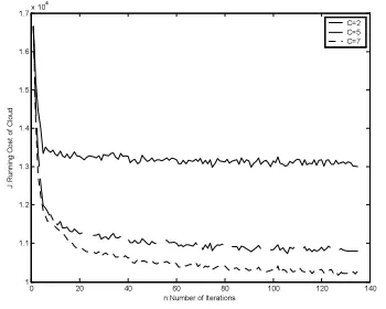
[image:8.595.315.490.442.577.2]

J :R u n n in g C o s t o f C lo u d C=2 C=5 C=7

Figure 3: Iterations Of Running Cost J Over Different Load Level C.

First, during the learning process of the optimization algorithm, the relationship between the number of load levels and the iteration results of the running cost J is validated in fig. 3. The horizontal axis means the number of iterations n, and the vertical axis means the running cost of the cloud computing platform J. The solid line, dashed line, and dotted line stand for the change trends of J over

the number of iterations when

C

₌

₂

_,

C

₌

5

_,

7

C

₌

respectively, and three lines start iteration

from the same initial resource scheduling strategy. In fig. 3, we can see that the higher the number of C, the better the results of the optimization for J. But the time for algorithm learning increases fast when the number of C increases.

Then, the effort of the optimization on the resource balance is showed in the fig. 4. Let

n

resba

_{be the value which can reflect the resource}

balance of the n-th iteration, and it can be obtained from the equations (23), (24) and (25).

(

)

,

1

1 /

M

k m k

m

averageres

M

Sused

=

=

⋅

∑

(23)

(

)

1/ 2 ' 2 , , 1 m K K

m state k m k k

k

resb urc Sused averageres + =   =_ ⋅ − _ 

∑

 (24) ,

1 1 1

/

m

M NS NS

n m state ns ns

m ns ns

resba

resb

t

t

= = =



 



=

_

⋅

_{ }

_



 



∑ ∑

∑

(25)

The value of

averageres

k means the average

used resources k of all servers. The value of

, m

m state

resb

_{means the effort of resource balance of}

server m in

state

m.

0 20 40 60 80 100 120 140 3000 3500 4000 4500 5000 5500 6000

n:Number of Iterations

[image:8.595.102.277.470.610.2]

re s ba: E ff or t of R es our c e B alanc e C=2 C=5 C=7

Figure 4: Iterations Of Effort On Resource Load Balance Resba Over Different Load Level C.

In fig. 4 the horizontal axis means the number of iterations n, and the vertical axis means the effort of

resource balance

resba

n. The solid line, dashed

line, and dotted line stand for the change trends of

n

resba _{over the number of iterations when}

_C

₂

=

,

5

C

₌

_,

C

₌

7

_{respectively, and three lines start}

iteration from the same initial resource scheduling policy. In fig. 4, we can see that the higher the number of C, the better the results of the

optimization for

resba

n which means that the

good and the resource utilization improves. But the time for algorithm learning increases fast when the number of C increases.

Next, we should give the range of J to validate the proposition which we proposed in the convergence proof about the boundedness of J. The

value of C is fixed as 5. Let

J

ub be the running cost

of the cloud network when all the resources in the

servers have been used, we can see that

J

≤

J

ub is

always right, and

J

ub can be the upper bound of J.

Then, we iterate the running cost of the cloud computing platform J from different initial

strategies

rescm

1 ,

rescm

₂ and

rescm

₃

respectively. And the convergence of running cost J and the scheduling strategies can be seen in fig. 5 and table 1 respectively. The value of C is still fixed as 5.

0 50 100 150

1 1.2 1.4 1.6 1.8 2 2.2x 10

4

n:Number of Iterations

J

:R

u

nn

in

g

C

o

s

t

of

C

lo

ud

[image:9.595.308.506.160.379.2]

rescm1 iteration rescm2 iteration rescm3 iteration

Figure 5: Covergence Of Running Cost J.

In fig. 5, the solid line, the dashed line and the dotted line stand for the change trends of J which

iterated from different initial policies

rescm

1 _,

2

rescm

_and

rescm

_{3, respectively. We can see}

that three lines merged over the number of iterations which means that the running cost J iterated from different initial strategies converge to the same value.

In table 1, we can see that the scheduling strategies which iterate from different initial

policies

rescm

1 ,

rescm

₂ and

rescm

₃

respectively converge to three similar strategies. They should converge to the same strategy in theory, but there are measurement errors. So the convergence of the resource scheduling policy can be validated by table 1.

Fig. 5 and table 1 show that the job scheduling optimization algorithm is convergent.

Table 1: Convergence Of Scheduling Policies

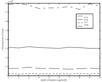
At last, after the algorithm learning, a new system log segment of 10 months is input into our system to validate the job scheduling policy generated by the optimization algorithm, and the effort of CUA is also shown.

1 2 3 4 5 6 7 8 9 10 1

1.1 1.2 1.3 1.4 1.5 1.6 1.7 1.8x 10

4

Month of System Log(month)

J

:R

un

n

ing

C

o

s

t

o

f

C

lo

u

d

[image:9.595.98.277.352.499.2]

C=2 C=5 C=7 CUA

Figure 6: Optimization Algorithm’s Validation On Running Cost J.

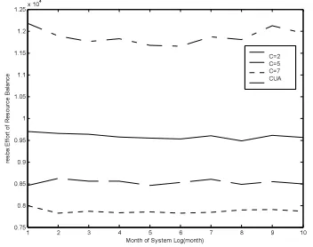
In fig. 6 and fig. 7, the horizontal axises mean the month of the system log segment, and the vertical axises mean the running cost of cloud computing platform J and the effort of resource balance resba respectively. The solid lines stand for the change trends of J and resba of the job scheduling strategy

generated by optimization algorithm of

C

₌

2

over

the month of log segment respectively. The dashed lines and dotted lines are corresponding to the

[image:9.595.319.491.448.587.2]

dashed dotted lines stand for the change trends of J and resba of CUA over the month of log segment respectively.

1 2 3 4 5 6 7 8 9 10

0.75 0.8 0.85 0.9 0.95 1 1.05 1.1 1.15 1.2 1.25x 10

4

Month of System Log(month)

re

s

b

a

:Ef

fo

rt

o

f

R

e

s

o

u

rc

e

B

a

la

n

ce

[image:10.595.100.276.172.311.2]

C=2 C=5 C=7 CUA

Figure 7: Optimization Algorithm’s Validation On Effort Of Resource Balance.

Fig. 6 and fig. 7 show that the final strategy generated by the optimization algorithm can not only improve the resource utilization, but also make the running cost of multimedia cloud computing network minimum compared with commonly used algorithm. But there is an unavoidable problem, since the job scheduling policy is generated by learning the old data record, the policy may become inappropriate when the user environment change greatly. We input the newest data record of long enough time to the optimization algorithm for relearning to solve this problem when two recent results of the scheduling policy are very different.

5. CONCLUSION AND FUTURE WORK

Cloud computing has brought great impact to the ordinary systems, and as a key part of the cloud computing, the job scheduling strategy problem is a challenging issue. In this study, we present a job scheduling policy with considering shared resources for the cloud computing, then an optimization algorithm is proposed to optimize the key matrix parameter of the job scheduling policy to obtain the optimal policy for the system, and the convergence proof of the optimization is also given. The numerical validation can support that the optimized strategy is able to minimize the running cost of the cloud computing platform and improve the resource utilization.

But there are still some issues about the optimization that will be explored in our future research. First sometimes the jobs arrive at the cloud computing platform in a short period of time, the job scheduling strategy should support scheduling many job to the servers one time.

Second, the estimation of the resource requirements of a job should be accurate, and the value may include two parts: maximum resource requirements to determine whether the server is able to serve the job and average resource requirements to participate the job scheduling policy, it can help improve the efforts of the job scheduling policy.

ACKNOWLEDGMENT

This work was partly supported by National Natural Science Foundation of P.R. China under grant No.61074033 and Doctoral Fund of Ministry of Education of P.R. China under grant No.20093402110019.

REFRENCES:

[1] X.F. Jiang, H.S. Xi, Q. Chen, J. Li and F.B. Li,

“Resources Scheduling Optimization for Multi-service Cloud Computing Based on Queuing

Networks,” Annual International Conference

on Cloud Computing and Virtualization, 2010, pp. 108-114.

[2] W.W. Zhu, C. Luo, J.F. Wang, S.P. Li,

“Multimedia Cloud Computing,” IEEE Signal

Processing Magazine, vol. 28 , 2011, pp. 59-69.

[3] Chaisiri, S., Lee, B. and Niyato, D.,

“Optimization of Resource Provisioning Cost in Cloud Computing,” IEEE Transactions on Services Computing, vol. 5, pp. 164-177, 2011.

[4] K.Q. Xiong and Perros H., “Service

Performance and Analysis in Cloud

Computing,” Services - I, 2009 World

Conference, 2009, pp. 693-700.

[5] X.H. Li, Y. Li, T.C. Liu, J. Qiu and F.C. Wang,

“The Method and Tool of Cost Analysis for

Cloud Computing,” Cloud Computing, 2009.

CLOUD '09. IEEE International Conference, 2009, pp. 93-100.

[6] Marcos Dias de Assunção · Alexandre di

Costanzo · Rajkumar Buyya, “A cost-benefit analysis of using cloud computing to extend

the capacity of clusters,” Cluster Comput

(2010) , 2010, vol. 13, pp. 335-347.

[7] W.Y. Zeng, Y.L. Zhao and J.W. Zeng, “Cloud

service and service selection algorithm

research,” Proceedings of the first

ACM/SIGEVO Summit on Genetic and Evolutionary Computation, 2009, pp. 1045-1048.

[8] L.Q. Li, “An Optimistic Differentiated Service

Job Scheduling System for Cloud Computing

Service Users and Providers,” Multimedia and

International Conference, 2009, pp. 295-299.

[9] Jamal, M.H., Qadeer, A., Mahmood, W. and

Waheed, A., and Ding, J., “Virtual Machine Scalability on Multi-Core Processors Based Servers for Cloud Computing Workloads,”

Networking, Architecture, and Storage, 2009. NAS 2009. IEEE International Conference, 2009, pp. 90-97.

[10]C.H. Zhao, S.S. Zhang, Q.F. Liu, J. Xie and

J.C. Hu, “Independent Tasks Scheduling Based on Genetic Algorithm in Cloud Computing,”

Wireless Communications, Networking and Mobile Computing, 2009. WiCom '09. 5th International Conference, 2009, pp. 1-4.

[11]M. Xu, L.Z. Cui, H.Y. Wang and Y.B. Bi, “A

Multiple QoS Constrained Scheduling Strategy of Multiple Workflows for Cloud Computing,”

Parallel and Distributed Processing with Applications, 2009 IEEE International Symposium , 2009, pp. 629-634.

[12]Sadhasivam S., Nagaveni N., Jayarani R. and

Ram R.V., “Design and Implementation of an Efficient Two-level Scheduler for Cloud

Computing Environment,” Advances in Recent

Technologies in Communication and Computing, 2009. ARTCom '09. International Conference, 2009, pp.884-886.

[13]Mustafizur Rahman, Rajiv Ranjan and

Rajkumar Buyya, “Cooperative and

decentralized workflow scheduling in global

grids,” Future Generation Computer Systems,

vol. 26, 2009, pp. 753-768.

[14]Marco A. S. Netto and Rajkumar Buyya,

“Resource Co-Allocation in Grid Computing

Environments,” Handbook of Research on P2P

and Grid Systems for Service-Oriented Computing: Models, Methodologies and Applications, vol. 1, 2010, pp. 476-494.

[15]B. Zhao and Y.B. Hua, “A Distributed Medium

Access Control Scheme for a Large Network of

Wireless Routers,” IEEE Transactions on

Wireless Communications, vol. 7, no. 5, May 2008, pp. 1614-1622.

[16]Raj Subbu and Arthur C. Sanderson,

“Modeling and Convergence Analysis of

Distributed Coevolutionary Algorithms,” IEEE

Transactions on System, Man, and Cybernetics, vol. 34, no. 2, 2002, pp. 806-822.

[17]Xi-Ren Cao, Stochastic learning and

optimization—A sensitivity-based approach,

Springer Science+Business Media, 2007, pp.

147-177.

[18]J. Kiefer and J. Wolfowitz, “Stochastic

Estimation of the Maximum of a Regression

Function,” The Annals of Mathematical

Statistics. Vol. 23, 1952, pp. 462-466.