Short Term Hydro-Thermal Scheduling using Artificial
Immunue System
C. Jena
Asst. Prof School of Electrical
Engg
KIIT University, BBSR
C.K.Panigrahi,
Ph.D.School of Electrical Engg
KIIT University, BBSR
M.Das
Research Scholar, School of Electrical
Engineering, KIIT University
M. Basu,
Ph.D.Dept of Power Engg Jadavpur University
ABSTRACT
Artificial Immune System is applied to determine the optimal hourly schedule of power generation in a hydrothermal system. A multi-reservoir cascaded hydroelectric system with a nonlinear relationship between water discharge rate, net head and power generation is considered. The water transport delay between connected reservoirs is taken into account. The transmission losses are also taken into consideration using loss coefficients. The developed algorithm is illustrated for a test system and the test results are compared with those obtained by using differential evolution and evolutionary programming technique. From numerical results, it is seen that artificial immune system based approach provides better solution.
Keywords:
Hydrothermal scheduling, cascaded reservoirs, artificial immune system
Nomenclature
si
a
,
b
si,c
si,d
si,e
si: cost curve coefficients ofi
ththermal unit
sim
: output power of
i
th thermal unit at timem
min
si
,
max
si
: lower and upper generation limits for
i
th thermal unithjm
: output power of
j
th hydro unit at timem
min
hj
,
max
hj
: lower and upper generation limits for
j
th hydro unitDm
: load demand at time
m
Lm
: transmission loss at time
m
hjm
Q
: water discharge rate of
j
th reservoir at timem
min
hj
Q
,
max
hj
Q
: minimum and maximum water
discharge rate of
j
th reservoirhjm
V
: storage volume of
j
th reservoir at timem
min
hj
V
,
max
hj
V
: minimum and maximum storage volume
of
j
th reservoirj
C
1,
C
2j,C
3j,C
4j,C
5j,C
6j: power generationcoefficients of
j
th hydro unithjm
: inflow rate of
j
th reservoir at timem
uj
R
: number of upstream units directly above
j
th hydro planthjm
S
: spillage of
j
th reservoir at timem
lj
t
: water transport delay from reservoir
l
toj
:
h
number of hydro generating units
s
: number of thermal generating units
m
, M : time index and scheduling period1.
INTRODUCTION
Optimum scheduling of generation in a hydrothermal system is of great importance to electric utility systems. With the insignificant marginal cost of hydroelectric power, the problem of minimizing the operational cost of a hydrothermal system essentially reduces to that of minimizing the fuel cost for thermal plants under the various constraints on the hydraulic and power system network.
The main constraints include: the time coupling effect of the hydro sub problem, where the water flow in an earlier time interval affects the discharge capability at a later period of time, the cascaded nature of the hydraulic network, the varying hourly reservoir inflows, the physical limitations on the reservoir storage and turbine flow rate, the varying system load demand and the loading limits of both thermal and hydro plants.
more tractable. Some of these solution methods are mathematical decomposition [1], network flow [2], dynamic programming [3], deterministic optimization algorithm [4], lagrangian relaxation [5] and benders decomposition [6]. With the emergence of artificial and computational intelligence technology, attention has been gradually shifted to applications of such technology-based approaches to handle the complexity involved in real world problems. Stochastic search algorithms such as simulated annealing technique [7], evolutionary programming technique [8], genetic algorithm [9]-[10] and differential evolution [11] have been applied separately for optimal hydrothermal scheduling problem and circumvented the above mentioned weakness.
Artificial immune system (AIS) [12]-[18] has emerged in the 1990s as a new branch in computational intelligence. AIS is inspired by immunology, immune function and principles observed in nature. It is now interest of many researchers and has been successfully used in power system optimization problems [19]-[21].
This paper proposes AIS algorithm for short-term optimal scheduling of generation in a hydrothermal system which involves the allocation of generation among the multi-reservoir cascaded hydro plants and thermal plants with nonsmooth fuel cost function so as to minimize the fuel cost of thermal plants while satisfying the various constraints on the hydraulic and power system network. To validate the AIS-based hydrothermal scheduling algorithm, the developed algorithm has been illustrated for a test system [9]. The test results are also compared with those obtained by using of differential evolution (DE) and evolutionary programming (EP) technique. From numerical results, it is found that the proposed AIS based approach provides better solution.
2.
PROBLEM FORMULATION
The hydrothermal scheduling problem is aimed to minimize the fuel cost of thermal plants, while making use of the availability of hydro power as much as possible. The objective function and associated constraints of the hydrothermal scheduling problem are formulated as follows.
2.1 Objective Function
The fuel cost function of each thermal generating unit considering valve-point effects is expressed as the sum of a quadratic and a sinusoidal function. The total fuel cost in terms of real power output can be expressed as
1 1 min 2sin
m i sim si si si sim si sim si si se
d
c
b
a
f
(1) Affinity=f
1
( 2)2.2 Constraints
(i) Power Balance Constraints:
The total active power generation must balance the predicted power demand and transmission loss, at each time interval over the scheduling horizon
0
1 1
Lm Dm j hjm i sim h s
m
(3)The hydroelectric generation is a function of water discharge rate and reservoir water head, which in turn, is a function of storage.
j hjm j hjm j hjm hjm j hjm j hjm j
hjm
C
V
C
Q
C
3V
Q
C
4V
C
5Q
C
62 2 2
1
h
j
m
(4)
(ii) Generation Limits:
max min
hj hjm
hj
j
hm
(5) and max min si simsi
i
s,m
(6)(iii) Hydraulic Network Constraints
The hydraulic operational constraints comprise the water balance equations for each hydro unit as well as the bounds on reservoir storage and release targets. These bounds are determined by the physical reservoir and plant limitations as well as the multipurpose requirements of the hydro system. These constraints include:
(a) Physical limitations on reservoir storage volumes and discharge rates,
max min
hj hjm
hj
V
V
V
j
h,m
(7)max min
hj hjm
hj
Q
Q
Q
j
h,m
(8)b) The continuity equation for the hydro reservoir network
uj lj lj R l t m hl t m hl hjm hjm hjm hjm mhj
V
Q
S
Q
S
V
1 1
h
j
3.
ARTIFICIAL IMMUNUE SYSTEM
The immune system of vertebrates including human is composed of cells, molecules and organs in the body which protect the body against infectious diseases caused by foreign pathogens such as viruses, bacteria, etc. To perform these functions, the immune system has to be able to distinguish between the body’s own cells as the self cells and foreign pathogens as the non-self cells or antigens. After distinguishing between self and non-self cells, the immune system has to perform an immune response in order to eliminate non-self cell or antigen. Antigens are further categorized in order to activate the suitable defense mechanism and at the same time, the immune system also developed a memory to enable more efficient responses in case of further infection by the similar antigen.Clonal selection theory explains how the immune system fights against an antigen. It establishes the idea that only those cells which recognize the antigen, are selected to proliferate. The selected cells are subjected to an affinity maturation process which improves their affinity to the selected antigens.
Clonal selection operates both on B-lymphocytes or B cells produced by the bone marrow and T-lymphocytes or T cells produced by the thymus. When the body is exposed to an antigen, B cells would respond to secrete specific antibodies to the particular antigen. Thereafter, a second signal from the T-helper cells, a subclass of T cells, would then stimulate the B cell to proliferate and mature into terminal (non-dividing) antibody secreting cells called plasma cells. In proliferation, clones are generated in order to achieve the state plasma cells as they are the most active secretors of the antibodies at a larger rate than rate of antibody secretion by the B cells. The proliferation rate is directly proportional to the affinity level i.e. higher the affinity level of B cells more clones is generated. Clones are mutated at a rate inversely proportional to the antigen affinity i.e. clones of higher affinity are subjected to less mutation compared to those which exhibit lower affinity. This process of selection and mutation of B cells is known as affinity maturation.
T cells do not secrete antibodies but play a central role in the regulation of the B cell response and are the most excellent in cell mediated immune responses. Lymphocytes, in addition to proliferating into plasma cells, can differentiate into long-lived B memory cells. These memory cells circulate through the blood, lymph and tissues, so that when exposed to a second antigenic stimulus, they commence to differentiate into large lymphocytes which are capable of producing high affinity antibody, preselected for the specific antigen that had stimulated the primary response.
Artificial immune system (AIS) mimics these biological principles of clone generation, proliferation and maturation. The main steps of AIS based on clonal
selection principle are activation of antibodies, proliferation and differentiation on the encounter of cells with antigens, maturation by carrying out affinity maturation process, eliminating old antibodies to maintain the diversity of antibodies and to avoid premature convergence, selection of those antibodies whose affinities with the antigen are greater.
In order to emulate AIS in optimization, the antibodies and affinity are taken as the feasible solutions and the objective function respectively. Real number is used to represent the attributes of the antibodies.
Initially, a population of random solutions is generated which represent a pool of antibodies. These antibodies undergo proliferation and maturation. The proliferation of antibodies is realized by cloning each member of the initial pool depending on their affinity. In minimization problem, a pool member with lower objective value is considered to have higher affinity. The proliferation rate is directly proportional to the affinity of the antibodies. The maturation process is carried through hyper-mutation which is inversely proportional to the antigenic affinity of the antibodies. The next step is the application of the aging operator. This aging operator eliminates old antibodies in order to maintain the diversity of the population and to avoid the premature convergence. In this operator an antibody is allowed to
remain in the population for at most
generations. After this period, it is assumed that this antibody corresponds to local optima and must be eliminated from the current population, no matter what its affinity may be. During the cloning expansion, a clone inherits the age of its parent and is assigned an age equal to zero when it is successfully mutated i.e. when hyper-mutation improves its affinity.4.
DEVELOPMENT
OF
PROPOSED
ALGORITHM
In this section, an algorithm based on artificial immune system for solving hydrothermal scheduling problem is described below.
Let
h
s h h hj h
s si s
s
k
Q
Q
Q
Q
p
1,
2,...,
,...,
,
1,
2,...,
,...,
be a trial matrix designating thek
-th individual of a population to be evolved and
si si1,
si2,...,
sim,...,
si,
hj hj hjm hjhj
Q
Q
Q
Q
Q
1,
2,...,
,...,
. The elements
sim
and
Q
hjm are the power output of thei
th thermalunit and the discharge rate of the
j
th hydro plant at timem
. The range of the elements
sim andQ
hjmrespectively. Assuming the spillage in equation (9) to be zero for simplicity, the hydraulic continuity constraints are
1 1 1
1 0 m m hjm R l t m hl m hjm hj hj uj lj
Q
Q
V
V
hj
(10)
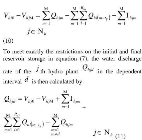
To meet exactly the restrictions on the initial and final reservoir storage in equation (7), the water discharge
rate of the
j
th hydro plantQ
hjd in the dependent intervald
is then calculated by
1 0 m hjm hj hjhjd
V
V
Q
+
1 1 1
m d m m hjm R l t m hl
Q
Q
u j lj hj
(11)
The dependent water discharge rate must satisfy the constraints in equation (8).
Also to meet exactly the power balance constraints in
equation (3), the thermal generation
sdgm of thedependent thermal generating unit
d
g can then be calculated using the following equation:
s hg d i i j hjm sim Lm Dm m sd 1 1
m
(12)The dependent thermal generation must satisfy the constraints in equation (6).
The cost function
f
is to be minimized. The algorithmic steps of AIS based on clonal selection principle are as follows:Step1) Antibody of size
is randomly generated. These must be feasible candidate solutions that satisfy the practical operating constraints.Step 2. The affinity value of each antibody in the population is evaluated using equation (2).
Step 3. The antibodies are cloned directly proportional to their affinities, giving rise to a temporary population of clones.
Step 4. The clones undergo maturation process through hyper-mutation mechanism whose rate is inversely proportional to their affinities. Each mutated clone must satisfy all the operating constraints.
Step 5. The affinities of the mutated clones are evaluated.
Step 6. Aging operator eliminates the antibodies and
mutated clones which have more than
generations from the current population.Step 7. Tournament selection is done to select a new population of the same size as the initial population from the antibodies and mutated clones which are remained after application of aging operator.
Step 8. If the maximum number of generations is reached, output the optimal solution i.e. the highest affinity value obtained so far and terminates the proposed algorithm. Otherwise, go back to Step 3.
5.
SIMULATION RESULTS
In this paper the performance of the proposed AIS-based hydrothermal scheduling problem is implemented using MATLAB 7 on a P-IV, 80 GB, 3.0 GHz personal computer. The proposed method has been applied to a test system which consists of a multi-chain cascade of four hydro units and three thermal units. The scheduling period is 24 hours with one hour time interval. The hydro sub-system configuration and network matrix including the water time delays are shown in figure 4, in the appendix. The load demand, hydro unit power generation coefficients, reservoir inflows, reservoir limits are given in tables 8, 9, 10 and 11 respectively in the appendix. The generation limits, cost coefficients of thermal units are given in table 12 in the appendix.
The problem is solved by using AIS algorithm. Here,
the population size
and the maximum iterationnumber
max are taken as 50 and 400 respectively forthe test system under consideration.
To validate the proposed AIS based approach, the same test system is solved using differential evolution (DE) and evolutionary programming (EP) technique.
In case of DE, the population size (
), scaling factor(
F
) and crossover constant (C
R) have been selected [image:4.595.49.280.106.334.2]as 500, 0.35 and 1.0. The population size is taken 50 in case of EP. Maximum number of generations has been selected 400 for both DE and EP.
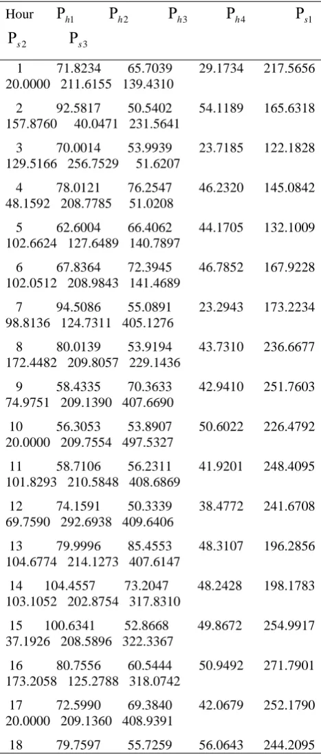
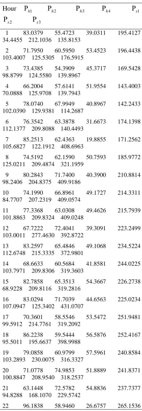
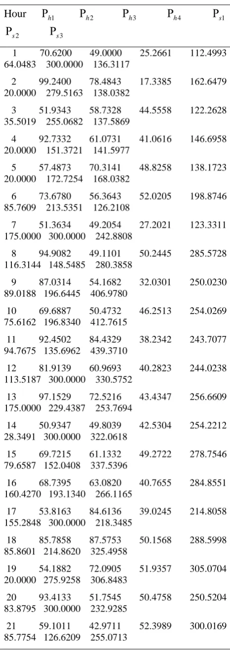
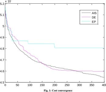
Table 1 shows the total cost obtained from AIS, DE and EP. The determined hydrothermal generation schedules and water discharge rates by using proposed AIS algorithm are shown in tables 2 and 3. The determined hydrothermal generation schedules and water discharge rates by using DE are given in tables 4 and 5. The determined hydrothermal generation schedules and water discharge rates by using EP are summarized in tables 6 and 7. Table 1 reveals that AIS has achieved lowest minimum cost. Figure 1 shows the cost convergence obtained from AIS, DE and EP.
Table 1: Comparison of cost
Method
Cost
( $)
AIS
45433
DE
45969
[image:5.595.50.284.210.760.2]EP
48062
Table 2: Hydrothermal generation (MW) schedule using AIS
Hour
h1
h2
h3
h4
s12
s
s31 71.8234 65.7039 29.1734 217.5656 20.0000 211.6155 139.4310
2 92.5817 50.5402 54.1189 165.6318 157.8760 40.0471 231.5641
3 70.0014 53.9939 23.7185 122.1828 129.5166 256.7529 51.6207
4 78.0121 76.2547 46.2320 145.0842 48.1592 208.7785 51.0208
5 62.6004 66.4062 44.1705 132.1009 102.6624 127.6489 140.7897
6 67.8364 72.3945 46.7852 167.9228 102.0512 208.9843 141.4689
7 94.5086 55.0891 23.2943 173.2234 98.8136 124.7311 405.1276
8 80.0139 53.9194 43.7310 236.6677 172.4482 209.8057 229.1436
9 58.4335 70.3633 42.9410 251.7603 74.9751 209.1390 407.6690
10 56.3053 53.8907 50.6022 226.4792 20.0000 209.7554 497.5327
11 58.7106 56.2311 41.9201 248.4095 101.8293 210.5848 408.6869
12 74.1591 50.3339 38.4772 241.6708 69.7590 292.6938 409.6406
13 79.9996 85.4553 48.3107 196.2856 104.6774 214.1273 407.6147
14 104.4557 73.2047 48.2428 198.1783 103.1052 202.8754 317.8310
15 100.6341 52.8668 49.8672 254.9917 37.1926 208.5896 322.3367
16 80.7556 60.5444 50.9492 271.7901 173.2058 125.2788 318.0742
17 72.5990 69.3840 42.0679 252.1790 20.0000 209.1360 408.9391
18 79.7597 55.7259 56.0643 244.2095
174.5975 214.8082 316.8189
19 64.4397 62.6780 52.4424 224.2113 74.4668 209.8371 407.0209
20 64.4639 69.4904 56.4943 257.5805 94.2513 207.3418 317.9596
21 90.2071 47.8455 57.5221 268.1632 20.2087 40.5135 408.9404
22 87.9591 65.5452 43.1193 296.4617 104.2330 210.5357 58.7539
23 58.4318 46.6280 54.0516 290.9288 145.1913 126.1552 137.4614
24 57.4695 51.7444 55.4865 275.0541 100.7017 40.0000 229.6560
Table 3: Hourly plant discharge (
10
4m
3) using AISHour
Q
h1Q
h2Q
h3Q
h41 7.4923 8.6492 23.1053 13.6956
2 11.3952 6.2747 15.1734 9.6111
3 7.2206 6.6299 29.2546 8.5292
4 8.4289 10.3139 15.3465 9.1301
5 6.2359 8.5376 29.8321 13.6244
6 6.9477 9.7434 13.0899 11.3238
7 12.4796 6.9984 21.4446 11.4096
8 9.1656 6.9133 16.0919 16.5749
9 5.8679 9.8137 16.6103 19.3368
10 5.4754 7.0770 13.1506 13.9435
11 5.6215 7.2544 18.2051 16.8570
12 7.4604 6.2069 18.7023 15.2781
13 8.2511 13.1254 14.8473 10.4395
14 14.1109 10.6643 15.2593 10.1064
15 12.6908 7.0503 14.7310 15.6278
16 8.4030 8.1036 14.5500 17.4989
17 7.1689 9.7900 19.6052 14.8417
18 8.1472 7.6097 14.9234 13.9514
19 6.1021 9.0471 17.2119 11.8128
20 6.0932 10.8484 14.8819 14.9923
21 9.8963 7.0540 14.7944 16.3219
22 9.5944 10.0802 20.2685 20.0000
23 5.4512 6.7675 16.6281 20.0000
[image:5.595.317.535.286.737.2]Table 4: Hydrothermal generation (MW) schedule using DE
Hour
h1
h2
h3
h4
s12
s
s31 83.0379 55.4723 39.0311 195.4127 34.4455 212.1036 135.8153
2 71.7950 60.5950 53.4523 196.4438 103.4007 125.5305 176.5915
3 73.4385 54.3909 45.3717 169.5428 98.8799 124.5580 139.8967
4 66.2004 57.6141 51.9554 143.4003 70.0888 125.9708 139.7943
5 78.0740 67.9949 40.8967 142.2433 102.0390 129.9381 114.2687
6 76.3542 63.3878 31.6673 174.1398 112.1377 209.8088 140.4493
7 85.2513 62.4363 19.8855 171.2562 105.6827 122.1912 408.6963
8 74.5192 62.1590 50.7593 185.9772 125.0211 209.4874 321.1959
9 80.2843 71.7400 40.3900 210.8814 98.2406 204.8375 409.9186
10 74.1990 66.8961 49.1727 214.3311 84.7707 207.2319 409.0574
11 77.3368 63.0308 49.4626 215.7939 101.8863 209.8324 409.0248
12 67.7222 72.4041 39.3091 223.2499 103.0011 277.4630 392.8722
13 83.2597 65.4846 49.1068 234.5224 112.6748 215.3335 372.9801
14 68.6633 60.5684 41.8581 244.0225 103.7971 209.8306 319.3603
15 82.7858 65.3513 54.3667 226.2738 68.9228 209.8116 319.2816
16 83.0294 71.7039 44.6563 225.0234 107.0947 125.3402 431.0707
17 70.3601 58.5546 53.5472 251.9481 99.5912 214.7761 319.2092
18 86.2238 59.5444 56.5876 252.4167 95.5011 195.6637 398.9988
19 79.0858 60.9799 57.5961 240.8584 103.2893 230.0075 316.3327
20 71.0778 74.9853 51.8889 241.8371 100.8847 208.9540 318.2537
21 63.1448 72.5782 54.8836 237.7377 94.8288 168.1070 229.5742
22 96.1838 58.9460 26.6757 265.1536
70.5463 209.6319 139.7170
23 79.5338 56.2234 52.7110 285.2911 102.4098 121.9618 159.5101
[image:6.595.313.538.142.618.2]24 89.4889 67.9722 55.6455 286.4694 127.4616 40.6164 139.7675
Table 5: Hourly plant discharge (
10
4m
3) using DEHour
Q
h1Q
h2Q
h3Q
h41 9.3900 6.9497 21.2930 11.3572
2 7.4625 7.6591 15.8795 12.3978
3 7.6448 6.6613 18.1371 10.7714
4 6.6101 6.9412 14.5708 9.2545
5 8.3409 8.4337 19.1058 10.1961
6 8.1719 7.7006 21.0849 12.1472
7 9.8868 7.6118 22.8905 11.3632
8 8.0287 7.7196 11.1866 12.0963
9 8.9669 9.5187 19.0729 14.6682
10 7.8782 8.7747 16.1337 14.4444
11 8.2332 8.0673 16.0728 13.7218
12 6.6974 9.6979 19.4848 13.4565
13 8.9093 8.5795 16.4476 15.0548
14 6.6904 7.7925 19.2375 15.7018
15 8.5748 8.4857 12.3245 13.5412
16 8.5509 9.6270 19.1695 13.1287
17 6.7612 7.4541 15.7710 15.4584
18 8.9753 7.6602 12.1421 15.3920
19 7.9102 8.0769 14.4662 13.6510
20 6.8480 11.0746 17.9008 13.8923
21 5.8969 11.0149 16.6590 12.9495
22 10.8978 8.4443 23.4759 15.6595
23 8.0405 7.8971 16.9803 18.9149
Table 6: Hydrothermal generation (MW) schedule using EP
Hour
h1
h2
h3
h4
s12
s
s31 70.6200 49.0000 25.2661 112.4993 64.0483 300.0000 136.3117
2 99.2400 78.4843 17.3385 162.6479 20.0000 279.5163 138.0382
3 51.9343 58.7328 44.5558 122.2628 35.5019 255.0682 137.5869
4 92.7332 61.0731 41.0616 146.6958 20.0000 151.3721 141.5977
5 57.4873 70.3141 48.8258 138.1723 20.0000 172.7254 168.0382
6 73.6780 56.3643 52.0205 198.8746 85.7609 213.5351 126.2108
7 51.3634 49.2054 27.2021 123.3311 175.0000 300.0000 242.8808
8 94.9082 49.1101 50.2445 285.5728 116.3144 148.5485 280.3858
9 87.0314 54.1682 32.0301 250.0230 89.0188 196.6445 406.9780
10 69.6887 50.4732 46.2513 254.0269 75.6162 196.8340 412.7615
11 92.4502 84.4329 38.2342 243.7077 94.7675 135.6962 439.3710
12 81.9139 60.9693 40.2823 244.0238 113.5187 300.0000 330.5752
13 97.1529 72.5216 43.4347 256.6609 175.0000 229.4387 253.7694
14 50.9347 49.8039 42.5304 254.2212 28.3491 300.0000 322.0618
15 69.7215 61.1332 49.2722 278.7546 79.6587 152.0408 337.5396
16 68.7395 63.0820 40.7655 284.8551 160.4270 193.1340 266.1165
17 53.8163 84.6136 39.0245 214.8058 155.2848 300.0000 218.3485
18 85.7858 87.5753 50.1568 288.5998 85.8601 214.8620 325.4958
19 54.1882 72.0905 51.9357 305.0704 20.0000 275.9258 306.8483
20 93.4133 51.7545 50.4758 250.5204 83.8795 300.0000 232.9285
21 59.1011 42.9711 52.3989 300.0169 85.7754 126.6209 255.0713
22 54.0044 44.7356 53.5506 297.3547 20.0000 94.5109 310.3078
23 56.3437 79.3386 55.6198 296.1181 20.0000 40.0000 317.6570
24 58.8113 65.6309 58.9075 272.2352 74.6100 40.0000 239.8174
Table7: Hourly plant discharge (
10
4m
3) using EPHour
Q
h1Q
h2Q
h3Q
h41 7.3148 6.0000 28.9895 6.4197
2 14.2478 11.0414 25.9467 9.3072
3 5.0000 7.5649 16.3017 6.0000
4 11.6837 7.8038 16.9207 8.3103
5 5.7111 9.3281 10.6053 8.3344
6 7.9694 7.0626 12.7754 11.9744
7 5.0000 6.0124 30.0000 6.6604
8 12.8892 6.0000 14.1618 20.0000
9 10.7988 6.6461 30.0000 20.0000
10 7.4820 6.0000 14.2549 17.1550
11 12.0973 11.9966 18.3254 16.3921
12 9.3921 7.5743 17.6771 14.5921
13 15.0000 9.5945 16.3931 16.1929
14 5.0000 6.0000 28.2554 20.0000
15 7.1686 7.4292 11.7586 18.0830
16 6.8970 7.5969 18.9886 18.9905
17 5.0000 11.9054 19.2118 11.0084
18 9.2829 13.9822 14.4977 18.8956
19 5.0000 10.9031 11.9679 20.0000
20 10.7954 7.4358 15.0330 13.9259
21 5.6043 6.0272 10.1091 19.7012
22 5.0000 6.0000 16.2196 19.3475
23 5.2170 12.3770 10.0000 20.0000
24 5.4484 9.7185 12.1456 17.5741
Fig. 1: Cost convergence
6.
CONCLUSION
A novel approach based on artificial immune system has been presented to solve the short-term hydrothermal scheduling problem. Numerical results show that highly near-optimal solutions can be obtained by artificial immune system algorithm when compared with the differential evolution and evolutionary programming technique. The same problem can be solved using other optimization technique and can be compare with this technique
7.
REFERENCES
[1] M. V. F. Pereira and L. M. V. G. Pinto, “A decomposition approach to the economic dispatch of the hydrothermal systems”, IEEE Transactions on PAS, Vol. 101, No. 10, 1982, pp. 3851-3860.
[2] Q. Xia, N. Xiang, S Wang, B. Zhang and M. Huang, “Optimal daily scheduling of Cascaded plants using a new algorithm of non-linear minimum cost network flow”, IEEE Transactions on PWRS, Vol. 3, No. 3, 1988, pp. 929-935.
[3] S. Chang, C. Chen, I. Fong and P. B. Luh, “Hydroelectric generation scheduling with an effective differential programming”, IEEE Transaction on PWRS, Vol. 5, No. 3, 1990, pp. 737-743.
[4] A. A. F. M. Carneiro, S. Soares and P. S. Bond, “ A large scale of an optimal deterministic hydrothermal scheduling algorithm”, IEEE Transactions on PWRS, Vol. 5, No. 1, Feb. 1990, pp. 204-211.
[5] M. S. Salam, K. M. Nor, and A.R. Hamdam, “Hydrothermal scheduling based Lagrangian relaxation approach to hydrothermal coordination”, IEEE Transactions on PWRS, Vol. 13, No. 1, Feb. 1998, pp. 226-235.
[6] W. S. Sifuentes and A. Vargas, “Hydrothermal Scheduling Using Benders Decomposition: Accelerating Techniques”, IEEE Trans. on PWRS, Vol. 22, No. 3, Aug. 2007, pp. 1351-1359.
[7] K. P. Wong and Y. W. Wong, “Short-term hydrothermal scheduling part 1: simulated annealing approach”, IEE Proceedings Generation, Transmission and Distribution, 1994, Vol. 141, No.5, pp. 497-501.
[8] P. C. Yang, H. T. Yang and C. L. Huang, “Scheduling short-term hydrothermal generation using evolutionary Programming techniques”, IEE Proceedings Generation Transmission and Distribution, vol. 143, No. 4, July 1996, pp. 371-376.
[9] S. O. Orero and M. R. Irving, “A genetic algorithm modeling framework and solution technique for short term optimal hydrothermal scheduling”, IEEE Trans. on PWRS, Vol. 13, No. 2, May 1998.
[10]E. Gil, J. Bustos and H. Rudnick, “Short-term hydrothermal generation scheduling model using a genetic algorithm”, IEEE Trans. on PWRS, Vol. 18, No. 4, Nov. 2003, pp. 1256-1264.
[11]L. Lakshminarasimman and S. Subramanian, “Short-term scheduling of hydrothermal power system with cascaded reservoirs by using modified differential evolution”, IEE Proceedings – Generation, Transmission and Distribution, Volume 153, No. 6, November 2006, pp.693-700.
[12]S. Endoh, N. Toma, and K. Yamada, “Immune algorithm for n-TSP”, System, Man and Cybernetics, IEEE International Conference, vol. 4, 11-14 October, 1998, pp. 3844-3849.
0 50 100 150 200 250 300 350 400
4.5 4.6 4.7 4.8 4.9 5 5.1 5.2x 10
4
[13]L. N. de Castro, and F. J. Von Zuben: Artificial Immune Systems: Part I – Basic theory and Applications. Technical report, TR-DCA 01/99, Dec1999.
[14]L. N. de Castro and F. J. Zuben, “Learning and optimization using through the clonal selection principle”, IEEE Transactions on Evolutionary Computation, vol.6, no.3 pp. 239-251, 2002.
[15]G. Nicosia, V. Cutello, P. J. Bentley and J. Timmis: Artificial Immune Systems. Third International Conference (ICARIS 2004), Catania, Italy, LNCS, Springer-Verlag, vol.3239, 2004.
[16]V. Cutello, G. Morelli, G. Nicosia, and M. Pavone: Immune Algorithms with Aging Operators for the String Folding Problem and the Protein Folding problem. EvoCOP 2005, LNCS, vol. 3448, pp. 80-90, Springer, Heidelberg (2005).
[17]V. Cutello, G. Narzisi, G. Nicosia, and M. Pavone: Real coded Clonal Selection Algorithm for Global Numerical Optimization using a new Inversely Proportional Hypermutation Operator. The 21st Annual ACM
Symposium on Applied Computing, SAC 2006, Dijon, France, April 23-27, 2006, vol. 2, pp. 950-954. ACM Press, New York (2006).
[18]V. Cutello, G. Nicosia, M. Romeo and P. S. Oliveto: On the Convergence of Immune Algorithms. The First IEEE Symposium on Foundations of Computational Intelligence, FOCI 2007. IEEE Computer Society Press, Los Alamitos (2007).
[19]T. K. A. Rahman, S. I. Suliman and I. Musirin, “Artificial Immune –Based Optimization Technique for Solving Economic Dispatch in Power Systems”, Springer-Verlag, Berlin Heidelberg 2006, pp.338-345. [20]B. K. Panigrahi, S. R. Yadav, S. Agrawal and M. K.
Tiwari, “A clonal algorithm to solve economic load dispatch”, Electric Power System Research, 2006. [21]Gwo-Ching Liao, “Short-term thermal generation
scheduling using improved immune algorithm”, Electric Power System Research 76 (2006), pp. 360-373.
8.
APPENDIX
1
h
h2- - - - - -
Reservoir 1 - - - - --- - - - - - ---- - Reservoir 2
1
h
Q
Q
h23
h
Reservoir 3
- - -
- - -
3
h
Q
4
h
- - -
Reservoir 4 - - -
4
h
Q
Where:
hj
: natural inflow to
j
th reservoirhj
Q
: discharge of
j
th plantPlant 1
2 3
4
u
R
0
0
2
1
d t
2
3
4
0
[image:9.595.52.276.71.729.2]u R : no of upstream plants Figure 1: Hydraulic system network d
t
: time delay to immediate downstream plant Table 8: Load demand Hour D
(MW) Hour D
(MW) Hour D
(MW) 1 750 9 1090 17 10502 780 10 1080 18 1120
3 700 11 1100 19 1070
4 650 12 1150 20 1050
5 670 13 1110 21 910
6 800 14 1030 22 860
7 950 15 1010 23 850
[image:9.595.310.549.318.765.2]8 1010 16 1060 24 800
Table 9: Hydro power generation coefficients Plant 1
C
C
2C
3C
4C
5C
6 1 -0.0042 -0.42 0.030 0.90 10.0 -502 -0.0040 -0.30 0.015 1.14 9.5 -70
3 -0.0016 -0.30 0.014 0.55 5.5 -40
4 -0.0030 -0.31 0.027 1.44 14.0 -90
Table 10: Reservoir inflows ( 3 4
10
m
) Hour Reservoir 1 2 34 Hour Reservoir 1 2 3
4 Hour Reservoir 1 2 3
4 1 10 8 8.1 2.8 9 10 8 1
0 17 9 7 2
0 2 9 8 8.2 2.4 10 11 9 1
0 18 8 6 2
0 3 8 9 4
1.6 11 12 9 1
0 19 7 7 1
4 7 9 2 0
12 10 8 2 0
20 6 8 1 0 5 6 8 3
0
13 11 8 4 0
21 7 9 2 0 6 7 7 4
0
14 12 9 3 0
22 8 9 2 0 7 8 6 3
0
15 11 9 3 0
23 9 8 1 0 8 9 7 2
0
16 10 8 2 0
[image:10.595.47.286.71.226.2] [image:10.595.48.287.73.412.2]24 10 8 0 0
Table 11: Reservoir storage capacity limits, plant
discharge limits, reservoir end conditions (
3 4
10
m
) andplant generation limits (MW)
Pla
nt
min
V
V
maxV
iniV
endmin
Q
Q
max
hmin
hmax1 80 150 10
0
120 5 15 0 500
2 60 120 80 70 6 15 0 500
3 100 240 17
0
170 10 30 0 500
4 70 160 12
0
140 6 20 0 500
Table 12: Cost curve coefficients and operating limits of thermal generators
Unit
a
sb
sc
sd
se
smin
s
smax$/h $/MWh $/(MW)2h $/h rad/MW MW MW 1 100 2.45 0.0012 160 0.038 20 175
2 120 2.32 0.0010 180 0.037 40 300
3 150 2.10 0.0015 200 0.035 50 500
Transmission loss coefficients are given below:
B =
10
4
[ 0.34 0.13 0.09 -0.01 -0.08 -0.01 -0.02 0.13 0.14 0.10 0.01 -0.05 -0.02 -0.01 0.09 0.10 0.31 0.00 -0.11 -0.07 -0.05 -0.01 0.01 0.00 0.24 -0.08 -0.04 -0.07 per MW-0.08 -0.05 -0.11 -0.08 1.92 0.27 -0.02 -0.01 -0.02 -0.07 -0.04 0.27 0.32 0.00 -0.02 -0.01 -0.05 -0.07 -0.02 0.00 1.35]
B0 =