Kalman filtering techniques applied to the dynamic ship positioning problem

Kalman filtering techniques applied to the dynamic ship

positioning problem

AL-TAKIE, Adnan A.G.

Available from Sheffield Hallam University Research Archive (SHURA) at:

http://shura.shu.ac.uk/7118/

This document is the author deposited version. You are advised to consult the

publisher's version if you wish to cite from it.

Published version

AL-TAKIE, Adnan A.G. (1982). Kalman filtering techniques applied to the dynamic

ship positioning problem. Doctoral, Sheffield City Polytechnic.

Copyright and re-use policy

1W8

S heffield C ity Polytechnic Library

R

e fe r e n c e

o n l y

Fines are charged at 50p per hour

ProQuest Number: 10694143

All rights reserved

INFORMATION TO ALL USERS

The quality of this reproduction is dependent upon the quality of the copy submitted.

In the unlikely event that the author did not send a com plete manuscript and there are missing pages, these will be noted. Also, if material had to be removed,

a note will indicate the deletion.

uest

ProQuest 10694143

Published by ProQuest LLC(2017). Copyright of the Dissertation is held by the Author.

All rights reserved.

This work is protected against unauthorized copying under Title 17, United States C ode Microform Edition © ProQuest LLC.

ProQuest LLC.

789 East Eisenhower Parkway P.O. Box 1346

KALMAN FILTERING TECHNIQUES APPLIED TO THE DYNAMIC SHIP POSITIONING PROBLEM

by

ADNAN A G AL-TAKIE

A thesis, submitted to the Council for

National Academic Awards in partial fulfilment of the requirements for the decree of Doctor of Philosophy

The research was conducted at Sheffield City Polytechnic in collaboration with GEC

Electrical Projects Ltd, Rugby

KALMAN FILTERING TECHNIQUES APPLIED TO THE DYNAMIC SHIP POSITIONING PROBLEM

A A G Al-Takie Abstract

The dynamic ship positioning problem using Kalman filtering techniques is considered. The main components of the system are discussed. The ship dynamics, based on a linearised model, are represented by state equations. These equations involve low and high frequency subsystems. A simplified design procedure for the implementation of a Kalman filter

is described based on the linearised equations of motion. The Kalman filter involves a model of the system and is therefore particularly appropriate for separating the low and high frequency motions of the vessel. The filtering problem is one of estimating the low-frequency motions of the vessel so that control can be applied. An optimal ’ feedback control system simulation based on optimal stochastic control theory is used. The optimal control performance criterion weighting matrices Q, R were pre-selected and the optimal feedback gain matrix was computed. This control scheme involves the low-frequency part of the ship model. The Kalman filter has been simulated on a digital computer for different modelled operating conditions. The computer simulation results showing the behaviour and responses of the Kalman filter applied to the dynamic ship positioning problem were

investigated. The system dynamics vary as the weather conditions vary and can be classified from a calm sea condition (Beaufort number 5) to the worst condition (Beaufort number 9). Different tests involving systems modelling and filter mismatching have been carried out. Another field in which the robustness of a Kalman filter has been assessed involved a test in which the system observation noise covariance was increased keeping the filter with the usual noise information. Saving in both computation and computer storage

requirement were achieved using a form of semi-constant filter gain and reduced-order Kalman filter respectively.

System non-linearities have been considered and a non-linear control algorithm was proposed and implemented using an extended Kalman filter. These non-linearities involve the thruster dynamics and the associated low-frequency part of the system model.

CONTRIBUTION AND PUBLICATIONS

Summary of Contributions

1. Complete implementation of Kalman estimator together with optimal feedback control for "Wimpey Sealab" vessel.

2. In depth investigations into the non-linearities of main parts of the dynamic ship positioning systems.

3. Complete development of dynamic positioning control based on Kalman filtering and optimal feedback control for "Star Hercules" vessel.

Publications

1. AL-TAKIE, A A: "Development of a dynamic ship positioning

simulation", Research Report EEE/28/1979, Sheffield City Polytechnic.

2. AL-TAKIE, A A: "Documentation report on the selection of the optimal control performance criterion", Research Report, January 1980, Sheffield City Polytechnic

3. AL-TAKIE, A A: "Kalman filtering techniques applied to the dynamic positioning problem", Research Report EEE/53/May 1980, Sheffield City Polytechnic

4. AL-TAKIE, A A and GRIMBLE, M J: "Optimal control of non-linear stochastic systems with application to dynamic ship positioning",

International Conference on Systems Engineering, September 14-16, 1982,

Coventry (Lanchester)Polytechnic, UK.

5. GRIMBLE, M J and AL-TAKIE, A A: "Optimal control of non-linear

ACKNOWLEDGEMENTS

I would like to express my gratitude and sincere thanks to my super­

visor, Professor M J Grimble, for his guidance, valuable advice and encouragement all through the period of this research work.

The work described in this thesis was partially financed by the

British Science and Engineering Research Council for which the author is most grateful.

The work has been carried out in close liaison with GEC Electrical Projects, Rugby and I would particularly like to thank Mr D Wise for

his valuable technical advice.

Thanks due to Mr D Abraham, Head of Department of Electrical and Electronic Engineering, Sheffield City Polytechnic and to virtually

every member of his staff who have offered their help and suggestions with respect to difficulties.

My thankfulness is also extended to Dr R J Patton of the Department of Electrical Engineering, York University, for his help and advice on the software developments.

TABLE OF CONTENTS

page

ABSTRACT i

CONTRIBUTION AND PUBLICATIONS ii

ACKNOWLEDGEMENTS iii

CHAPTER 1 - GENERAL ASPECTS OF THE DYNAMIC POSITIONING 1 PROBLEM

1.1 General Introduction 1

1.2 Notch, PID Filtering and Control 8

1*3 Alternative, Kalman Filtering and

Stochastic Optimal Control Solution 9

1.4 Thesis Layout 13

CHAPTER 2 - MAIN PARTS OF THE DYNAMIC SHIP POSITIONING

SYSTEMS 15

2.1 Introduction 15

2.2 Thruster Devices 17

2.2.1 Introduction 17

2.2.2 Thruster used on "Wimpey Sealab" 20 2.2.3 Thruster used on "Star Hercules" 22

2.2.4 Thruster applied forces 27

2.3 Position and Heading Measurement Systems 28

2.4 Process and Measurement Noise Analysis 31

2.4.1 The Process Noise 33

2.4.2 The Observation Noise 34

CHAPTER 3 - THE SHIP MOTION 35

3.1 Introduction 35

3.2 Low-Frequency Dynamics 39

3.2.1 Introduction 39

3.2.2 Derivation of the Low-Frequency Dynamics 41 3.2.3 Low-Frequency Equations for "Wimpey

Sealab" vessel 43

3.2.4 Low-Frequency Equation for "Star Hercules"

vessel 48

3.3 High-Frequency Dynamics 49

3.3.1 Introduction 49

3.3.2 Development of the High-Frequency Model 50

CHAPTER 4 - THE STOCHASTIC OPTIMAL CONTROL PROBLEM 54

4.1 Introduction 54

4.2 Control Algorithm 57

4.3 Selection of the Performance Criterion Weighting

page

4.4 Simulations and Results 65

4.4.1 Case (a) 65

4.4.2 Case (b) 66

4.4.3 Case (c) 73

4.5 Concluding Remarks 76

CHAPTER 5 - LINEAR FILTERING/KALMAN FILTERING PROBLEM 82

5.1 Introduction 82

5.2 Kalman Algorithm 84

5.3 Implementations and Simulation Results 88

5.3.1 Software Description 88

5.3.2 Filter and Control Implementations

for "Wimpey Sealab" vessel 90 5.3.3 Filter and Control Implementations

for "Star Hercules" vessel 98

5.4 Concluding Remarks 107

CHAPTER 6 - PRACTICAL INVESTIGATION INTO THE USE OF KALMAN

FILTERING FOR DYNAMIC POSITIONING 109

6.1 Introduction 109

6.2 Reduced-Order Kalman Filter 110

6.3 Semi-Constant Gain Kalman Filter 112

6.4 Filter Mismatching 121

6.5 Reliability Tests 126

6.6 Concluding Remarks 129

CHAPTER 7 — NON-LINEAR FILTERING/EXTENDED KALMAN FILTER 130

7.1 Introduction 130

7.2 Non-Linear Filtering and Control 131

7.2.1 System Description including Thrusters

Non-Linearities 132

7.2.2 The Filtering Algorithm 136

7.2.3 The Control Algorithm 139

7.2.4 Simulation Results 140

7.3 Parameter Estimations 141

7.4 Concluding Remarks 150

CHAPTER 8 - OVERALL CONCLUSIONS 151

REFERENCES 155

CHAPTER 1

GENERAL ASPECTS OF THE DYNAMIC POSITIONING PROBLEM

1.1 General Introduction

Since the end of World War II, it has been increasingly realised that the seabed and rock beneath are rich in mineral resources which should be exploited. The best known example is the offshore oil reserves.

Initially, exploitation was limited to shallow water close to the shore but it has moved progressively into deeper water and less hospitable

locations. Early exploration for oil production was carried out from

fixed platforms. Inspection and maintenance work on fixed structures involve extensive use of diving services and lifting facilities. From these has arisen the need for the floating vessel with the necessary technique to keep it stationary with respect to some reference point. Recently many floating drilling rigs and drill ships have been intro­ duced and many of these are working in the North Sea. In addition to

drilling, offshore operations involve: (i) coring

(ii) surveying (iii) cable laying

(iv) dredging

(v) diving

(vi) fire fighting

The most significant limitation of using the conventional floating vessel

is the difficulty of anchoring in deep water. To overcome these

limitations, the concept of a dynamic positioning technique was intro­ duced. Dynamic ship positioning is defined as the technique for

point on the seabed without the use of anchoring systems. The second definition of dynamic positioning is that the vessel may be moving at controlled speed, which can be extended to include the tracking

problem.

The process of automatically controlling a ship or floating platform position and heading [li] £l9] over a preselected area is concerned with

providing the necessary thrust in appropriate quantity and direction to match the mean loads imposed on the vessel by environment and other forces. This will involve using:

(i) a combination of thruster mechanism and propulsion

(ii) position and heading measuring devices (iii) wind speed sensor

(iv) control computer

The design of an automatic position and heading control system for a vessel depends on the required criteria, which must be satisfied by the vessel and its control system (or computer control system) to

perform its mission, on the environmental conditions in the area where the vessel will operate and on the expected behaviours of the vessel for changing weather.

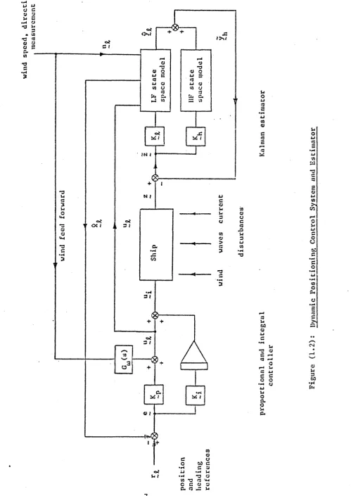
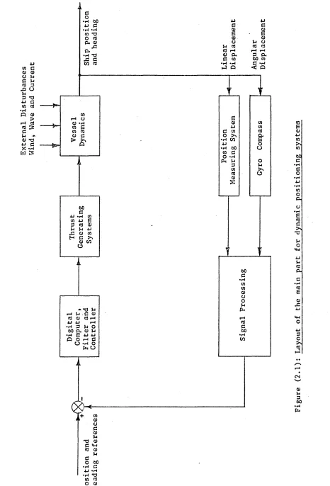
The control system is part of a closed loop system, schematically shown in Figure 1.1. The main components are:

(i) measurement subsystem, including all devices for generating the information to be processed by the computer,

(ii) the filter to attenuate the unwanted signals and to generate the required estimates for state feedback control,

(iii) the controller, of which the output is sent to the propulsors

(main propellers and other thrusters),

Ex te rn al di st ur ba nc es ■u c<u uu do a) % & T3_C •H 60 QJ »H

J-l 4-1

a) *h

to *H to «H

position.

This control scheme should be capable of:

(i) controlling the propulsors for maintaining a reference position

and heading under specified weather conditions (with the ability to react to changing weather conditions), with a maximum allowable radial position error of 3 per cent of the water depth,'

(ii) avoiding high-frequency fluctuations in the thrust demand (filtering problem) since this may cause unnecessary wear of the propulsors and waste of energy,

(iii) controlling the propulsors for changing the position or heading of the ship in case a new reference position or heading is selected.

Dynamic positioning systems with on-line computer control involve

one of the following [3C^ :

(i) Simplex computer control, where longer term or more accurate position keeping is necessary, such as for support purposes. This

fully automatic control system is an economic scheme and it normally comprises:

(a) one computer complete with monitoring unit and peripherals controllers

(b) one operator console, with full set-up, control and display

(c) one position measurement system

(d) set of environmental and attitude sensors

(ii) Duplex computer control, which is usually used for oil exploration drilling vessels, which is required to remain on station for long periods

of time.A Full automatic duplex dynamic positioning system comprises of:

(b) one operator console, with full set-up, control and display,

(c) two position measurement systems,

(d) two sets of environmental and attitude sensors.

The design of a vessel*s dynamic positioning system involves a

compromise between the two conflicting requirements of accuracy of position holding and the need to suppress the thrusters response to part of the wave motions. These external forces are assumed to consist of low-frequency and high-frequency forces. The thrusters response

to the first order high-frequency wave motions is oscillatory in nature, and involves an extra power demand and wear and tear of the

thrust-producing mechanisms, without any gains in counteracting vessel

motion due to the above waves and forces.

The accuracy of the dynamic positioning system will depend to a certain extent on the philosophy of the wave filter selection method and the corresponding controller design procedure. Thus, the amount of the

thrusters oscillations will depend on the wave filter attenuation and the controller bandwidth. Filtering for the dynamic positioning problem can be defined as the process of operating upon the corrupted

information (the noisy measured system output) to attempt to construct a signal which can be used for control purposes [l8j, [22]]. The control systems for the first dynamically positioned vessels [3lj,[30j included

Notch filters and PID controllers. Using such a scheme, the position measurement signal can be filtered out to obtain a comparatively good estimate of the low-frequency part of the vessel motions, and hence, control can be applied [23]• An introduction to Notch filter

Using the above conventional Notch filter scheme with PID control can cause some difficulties since a compromise should be made between improved filtering and good control system performance. Such diffi­

culties led to the use of the alternative Kalman filtering technique together with modern stochastic optimal control theory. The

Kalman-Bucy filter [58], Q>o], [47], [46] has assumed a role of ever increasing importance over recent years in the field of filtering and estimation of processes, and its applications in dynamic systems. Theoretically, the Kalman filter gives the unbiased, minimum variance estimation of the state vectors of a linear or linearised dynamic system when output measurements are provided which represent a

linear function of the system states with some additive white noise.

In practice, optimum performance will be very hard to realise since the information required to construct the Kalman filter is only

approximately known. Hence, to get the best filtering and estimation,

the Kalman filter has to be provided with as much information as possible concerning the noise statistics and system dynamics.

In dynamic vessel positioning the low-frequency part of the system

states are required to be estimated by the Kalman filter so that control can be applied. Kalman filter dynamics, based on the separation

theorem [2l] , [54] will involve a model of the actual low and high frequency part of the system dynamics (Figure 1.2), and hence, the estimated high-frequency state vectors can be ignored, while the estimated low-frequency states can be fed back to be used within the control loop. An introduction into the use of the Kalman-Bucy

filtering scheme and its applications to the dynamic positioning

wi nd sp ee d, di re ct io n . m ea su re me nt o* CM o? S I o 3 o

aj e_<3

vi a

01 o₃

J*< C.

►J 01 •fi i>^i rH₃ •3 3 O vi 2* 3vi 3 ' 3 33 f.. C.

= 3 -3_u 3 3 Vj O <vi 3_O •3_C

V C< I a 3 J

V + 1 N ? o-CO •H 3 t *3 3 3 a o c a .3_u 3

3 J

1

r

3 O 53C

•H_{VI Vl}3 ■ p4 •3 3

u_o u3_E •r. V) a 3 C 2 E 3 S*S <-4 3Vi 50 3VI C •*-i Vi₃

1.2 Notch, PIP Filtering and Control

Notch filters [99j , [103^3 have been developed and used in dynamic ship positioning for some years with relatively good results. If the control system were purely analogue 7 this filter would obviously be preferred. With digital processors available, other filter structures might yield

will be introduced in the next section. A Notch filter is often used in dynamic positioning problems to attenuate the high-frequency wave motion signals from the position measurement system. The Notch filter must be capable of providing a constant attenuation ratio either for a fixed sea wave resonant frequency or for a range of resonant frequencies. A typical range of Notch frequencies [5l] would be 0.06 Hz to 0.12 Hz

corresponding to Beaufort scale number 9 down to 5 (Appendix 2). To provide a wide band-stop characteristic it is necessary to use a cascaded system of Notch filters with each section tuned to a

particular resonant frequency [20] , [l3[]. In this application three such cascaded sections are normally used. The Notch filter transfer function can be defined jioij by:

additional advantages. A Kalman filter with such properties

bd _{S + 0)}2

H(s)

(

.

)

s + s + 01

A - 2d2 where:

Notch centre frequency (rad/sec)

b the 3 dB bandwidth of the Notch (rad/sec)

d the attenuation ratio at the Notch centre frequency The above parameters w, b and d can be used to describe the Notch network. For a three cascaded section of this network the above

transfer function H(s) can be written as i=n

where: n = 3 (for three cascaded sections), and:

o kjdj 2

s + A 9a? s + Wi

V ® ) = ~ —_{2 +} ---bi ---*■... .(1-3)_{j- S + 0)}

A - 2di

where:

ok the ith section centre frequency

b. _l the ith section 3 dB bandwidth

d. _l the ith section attenuation ratio

1.3 Alternative Kalman Filtering and Stochastic Optimal Control Solution

Considerable research has been devoted during the last twenty years to various problems in the estimation of the states of linear dynamic systems using system measurements corrupted by Markov

noise. The Kalman-Bucy filtering technique for such, applications has

been thoroughly examined in the literature. The optimal, continuous time filtering problem for the case of linear system dynamics, additive measurements and Gaussian white disturbance measurement noise was

first solved by Kalman (1960) [58] and Kalman and Bucy (1961) [6o] .

Specifically they considered the problem of finding the unbiased, minimal variance state estimate x(t) of the system state x(t) in the

presence of stochastic input disturbances and output measurement additive noise.

The problem of state estimation of noisy systems using Kalman filtering scheme requires a knowledge of the system structure and its parameters QT]. If the system is linear or linearised and its different parameters are

known, the solution is a straightforward application of Kalman

parameters may be unknown and hence it is necessary to estimate them together with the system states simultaneously. This parameter estimation problem requires the extension of the Kalman filtering

scheme to include the system non-linearity. This will involve the implementation of the extended Kalman filter. This form of

non-linear filter problem can be dealt with by constructing an

additional linear dynamic model corresponding to the unknown parameters. The parameter equations are added to the system model equations and the

combined states and parameter variables of this augmented model are to be estimated. Feedback control can be applied using the low-frequency part of the state estimates only (Figure 1.3). All the necessary information concerning the process and observation noise as well as

system inputs have to be fed into the proposed filter dynamics for good estimation and filtering accuracy. The non-linear filtering problem for systems with random inputs is of great importance in control

processes, especially in industrial situations. The Kalman filter has been proved to be efficient and reliable for many industrial

applications.

The Kalman filtering scheme and its application to the dynamic

positioning problem has been proposed by the Norwegians (Balchen et al, 1976 Balchen*s design involves a more complicated and

computationally inefficient form of filter in which some of the

high-frequency parameters were estimated. An alternative solution to the linear and non-linear Kalman filtering problems with their

applications to the dynamic ship positioning problem was proposed and

used by Grimble Q>l] , [49]] . The use of the proposed alternative solution of Kalman filtering combined with the optimal control theory to the dynamic positioning problem was part of a Case

EXTERNAL

<Kl

o

H

o

H

EHH

CO

P

PH

HW

CO

P

o

P

h

EH

g

o

11

and carried out by a team of researchers. This work on dynamic positioning using Kalman filtering was an extension of in depth

study of general filtering and control problems by Grimble [35], [33], [36] . The simulations were involved in some high-frequency parameter estimations to estimate some of the unknown parameters within the high-frequency dynamics using an extended Kalman filter [49]t [52] .

These estimated parameters are to affect the high-frequency block of the system dynamics structure which varies in accordance with

the weather and sea conditions (Beaufort 9 for the worst sea condition down to Beaufort 5 for calm sea).

The team research provided a basic design for the dynamic ship positioning problem using Kalman filtering techniques based on data available from the "Wimpey Sealab" vessel. The author produced a complete design for the implementation of Kalman filtering and optimal stochastic control with its applications to the dynamic positioning problem based on data from the new "Star Hercules"

vessel. This vessel has already been commissioned by GEC Electrical Projects Limited, Rugby. The author has also contributed to an

original idea in which a special form of extended Kalman filter has been used employing the optimal control loop within the low-frequency part of the vessel dynamics. This form of non-linear control

caters for the non-linearities within the low-frequency dynamics and deals specifically in detail with the non-linearity of the thruster

1.4 Thesis Layout

In the previous sections of Chapter 1, the overall dynamic vessel

positioning problem has been introduced and its usefulness for

exploitation processes and other industrial applications were outlined. An introduction for the use of Notch, or Kalman filtering techniques within the dynamic positioning control loop were finally drawn in

Sections 1.2 and 1.3 respectively.

Chapter 2 contains a brief description of the main basic parts of the dynamic positioning systems. This will include the overall system

structure, the systems for measuring the position of the vessel, the thrust producing devices (for both "Wimpey Sealab" and "Star Hercules" vessels) and finally, the general statistics of both the process and observation noise.

Chapter 3 includes the basic linearised mathematical equations representing both the low and high frequency motions of the vessel.

These differential equations have been formulated on.the basis of data obtained from a set of "tank-tunnel-tests" and carried out by GEC Electrical Projects Limited, Rugby. These data were provided for both

"Wimpey Sealab" and "Star Hercules" vessels. Finally, system matrices were summarised for control and system simulations.

In Chapter 4, Grimble1s approach for the selection of the Q and R control weighting matrices has been implemented and used within the problem of the dynamic ship positioning. A form of the separation

theorem has been used and the matrix Riccati equation was solved to calculate the optimal feedback gain matrix. Finally, the low-frequency

the selection of the optimal gain matrix for future design (Chapters

5, 6).

Chapter 5 contains the main design results for a complete implementation and installation of the dynamic positioning system on both "Wimpey

Sealab" and "Star Hercules" vessels using linear Kalman filtering and stochastic optimal control techniques. This chapter has been extended to include tests and investigations into the reliability and

robustness of the Kalman filter algorithm and its application to the dynamic ship positioning problem.

In Chapter 6 the reliability and goodness of the Kalman filter and its

application to the dynamic ship positioning are to be investigated and several tests to be carried out to examine the scheme robustness.

Chapter 7 deals mainly with the case of non-linear filtering and control. Non-linearities in both the high-frequency and low-frequency dynamics of the system were studied and an extended Kalman filter has been used.

Finally, in Chapter 8, all the design procedures and results were

CHAPTER 2

MAIN PARTS OF THE DYNAMIC SHIP POSITIONING SYSTEMS

2.1 Introduction

The design of on-line computer control of a vessel position and

heading under dynamic positioning control depends on certain criteria. These must be satisfied by the vessel and its control system in order

to perform its mission (drilling, diving, fire fighting, etc), in the environmental conditions in the area where the vessel will operate and on the expected behaviour of the vessel under these environmental conditions. In dynamic positioning only the vessel motion in the

horizontal plane (surge, sway and yaw) are controlled, where the ship will be regarded as a rigid body. The vessel motions induced by the

waves are oscillatory motions with frequencies equal to the wave frequencies. At the same time the vessel drift from its original position is due to forces induced by the wind and the current. The vessel motion is assumed to consist of a low-frequency component and a high-frequency component. To keep the vessel motions, induced by the

external forces, within the required allowable limits, the vessel is fitted with a set of thrusters (Section 2.2). Considering the

requirements and environmental conditions, it may be stated that the control system should be designed to accept the relatively high-frequency

motions without any counter-act measures, while the low-frequency motions should be reduced and controlled on the basis of the required

accuracy for the different applications within the dynamic positioning technique (Table No 2.1).

ACCURACY

3% Water depth

± 3 m, Heading ± 2°

Heading ±1°, Excursion 1.5 m maximum

± 15 metres ENVIRONMENTAL CONDITION

Current (knots) CO t-H r— 1

Weather up to severe gale or storm conditions

Waves (metres) 3.9 4.5 2.0 Wind (knots) 25 30 20 (U (6 4J C u td 60 H o C £3 CL H •H (=» cl •U 0 ■u 60 w C 60 e <u •H •H 60 e r-4 C CL •H <1) •H > SJ >-i U •H cr •H P o W 16

maintaining the position of a vessel above a reference point on the

seabed without the use of anchors. This is to be achieved by employing a set of active thrusters controlled by a computer. The

error within the position can be monitored using different kinds of measurement techniques. These measurements could be corrupted by noise.

The main components in the dynamic positioning systems are the thrusters, the measurement systems, filter and the computer control (Figures 2.1,

i

2.2). System input signals from wind sensor, gyro compass and position measurements are fed into the control system and its associated computer to produce a command signal to the thrusters for appropriate action.

This computer control system should be capable of:

(i) controlling the propulsors for maintaining a reference

position and heading under specified adverse weather conditions, with a maximum allowable radial position error of 3 per cent of water depth or 7 metres (whichever is the smaller in case of drilling), or

controlling the propulsors to maintain the vessel at a constant speed,

(ii) avoiding high-frequency fluctuations in the thrust demand since this may cause unnecessary wear of the propulsors and power consumption,

(iii) controlling the propulsors for changing the position or heading of the ship in case a new reference position or heading is selected.

In this chapter the thrusters, the measurement systems and the

associated noise will be considered in detail, while the control system and the related filtering are due to be considered later.

2.2 Thruster Devices 2.2.1 Introduction

The dynamic ship positioning system has been defined as the process of

Ex te rn al Di st ur ba nc es Wi nd , Wa ve an d Cu rr en p i i g o •H 60

p g

•H *H_{CO 73} O CO a, a)_X a. •H 73_{X c}

CO to

(0 »— 1 o 0)•r4 to E to CO 0) g > >> Q j 60 C p •H CO to p e

3 to 0) P p p

X i 0) CO

H c ^_{ai co} O

Jk

» 73 P i“H I-i C a) CO QJ CO «-t P 4- f-c •H - P o oo a. qj p

*P E p p

P c r—1 C c •H O Pn CJ

A

( g K

+ CO <u o c0) p T3 OJ G »P CO OJ P co 60 •p C_{p •H} •H 73 p P 3 c QJ QJ e 6 0) QJ

o p a

P CO CO CO cO I— 1 H rH <U a. P a. g CO 60 CO •H •rH C •rl o < Q

s

QJ co

P CO

G CO CO

o a,

•H CO E

P o

•H 60 CP

CO g

O *P

PP P_P o_p

Hydrophones beacons Acoustic system Vertical reference unit Acoustic Signal Processor 4—

1. Heading 2. Display

-£=- Acoustic signal processor heading Anemometer 1 Heciding 1 heading * display --Control Console and displays

MARCH 4 I Thruster input/output,-*^— Servos

equipment Vertical reference unit Dual-axis inclinometer Taut-wire system Taut-wire signal ii Thrusters

x

GEC 2050 T computer

heading display

Figure (2.2): Schematic Diagram of the Dynamic Positioning

set of thrust-producing devices. In a dynamically positioned system the forces required to overcome the effects of wind, waves and currents

are provided by propellers, and the vessel pre-selected position

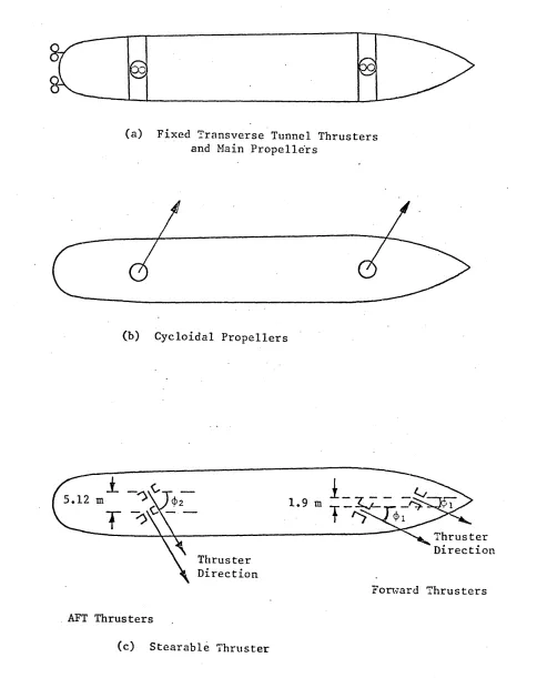
can be maintained by the use of a combination of thrusters and the main propulsion unit. Numerous types of thrusters are used for the dynamic ship positioning problem including plain propellers, ducted propellers

and cycloidal propellers [73l, (Figure 2.3). "When thrusters or

propellers are operated on a dynamic positioning vessel, the force and moment produced on the hull are not only due to the thrust devices

since interactions arise due to pressure changes on the hull, and these should be taken into consideration in some cases.

The principal types of thrust-producing units are: (i) screw propellers or thrusters,

(ii) cycloidal propellers (Voith Schneider units), (iii) pump type thrusters,

(iv) transverse tunnel thrusters, and

(v) steerable thrusters.

Figure (2.3) shows the most common configuration being used. The thrusters have both dead zone and saturation characteristics (the dead

zone for "Wimpey Sealab" is approximately 1-2% of the rated value of the thrusters [49))• The size of thrusters required is determined by

the largest magnitude of the steady drift forces and moments. To avoid the unnecessary wear and tear on the thrusters the control system should not attempt to compensate for the high cyclic vessel motions.

2.2.2 Thrusters used on "Wimpey Sealab11 vessel

George Wimpey and Company Limited have been involved in offshore drilling for many years. The dynamic positioning system, Figure 2.2,

(a) Fixed Transverse Tunnel Thrusters and Main Propellers

(b) Cycloidal Propellers

5.12 m _{1.9 m __ ^}

Thruster Direction

Thruster Direction

Forward Thrusters

AFT Thrusters

(c) Stearable Thruster

November 1972. The vessel (Figure 2.4) was the first British owned dynamically positioned drillship, and it has been used for site

investigation in addition to the drilling activities. "Wimpey Sealab" employs retractable a.c. motor driven thrusters with variable pitch

propellers (Figure 2.5). The vessel has two rotatable bow and two rotatable stern thrusters (capable of 360° rotation and each rated at

12.5 tonnes). The basic configurations of the thrusters are fully rotatable outboard propellers. Data from "Wimpey Sealab" were used

as the basic information for the implementation of the dynamic positioning technique throughout this work (Chapter 3).

2.2.3 Thrusters used on "Star Hercules" vessel

"Star Hercules" vessel (Figure 2.6) is the other vessel to be considered in this work. Data from the "Star Hercules" have been

obtained and used for design and simulation implementations.

The control thrust for the "Star Hercules" is provided by the main

engine and by two forward and one aft tunnel thrusters. Thruster locations used on "Star Hercules" are shown in Figure 2.7 and have the

following specifications:

The thrust

producing device Maximum thrust(tonne force) Thruster lever arms relativeto centre of gravity

Main Engine 28 (FWD)

19 (REV)

FWD.FWD Thrusters 5.1 31.03 metres

AFT.FWD Thrusters 9.1 28.62 metres

23

e

E

m

00

.—I

c

m

m

ciT

qs

-p

m

to

CO

O

CM

CO

26

2.2.4 Thrusters applied forces

The fore and aft thrusters on "Wimpey Sealab" act at angles <j>i and $2 relative to the vessels coordinates respectively (Figure 2.5). Let the thrusters forces be fj_ and f2 respectively for the fore and aft

thrusters. Then the thrusters force in the surge direction is:

f 1 cos + f2 cos (f>2

the total force in the sway direction is:

f 1 sin + fz sin <J>2

and the total force in the yaw direction is

fj&j sin (f^ - f2&2 sin (j>2

(

.

)

(

.

)

(2.3)

where = &2 = 10 metres ("Wimpey Sealab"). Hence, the per-unit equations in a matrix form (Appendix 1) will be:

surge force sway force

yaw force

cos ({), cos <f)t

sin (f)x

• 1 ^2 . .

— s m (p1 s m <J>2 _ sin (J>2

O 1 L_ 2f"

(2.4)

where:

f19 f2 are the per-unit values of f , f2 respectively. is the per-unit base length = 30 metres

0 < ^ < 1, 0 < < 1 and \

The matrix in equation (2.4) can be written in appropriate notation as:

~Yii _^12 COS (J)j cos 4>2

Y = ^21 Y22 = sin (f)x sin d)₂

- ^31 ^32 - - T ~^'1 sin * A-*1 _ _{t ^ J}

2.3 Position and Heading Measurement Systems

Dynamic positioning system is basically the technique in which control signals can be applied to propellers and thrusters for specific action

based on information concerning position and heading deviations from the pre-determined limits. In recent years the need for dynamic positioning has been increased by the problems associated with oil

exploration and production. With these applications, accuracy will be one of the main requirements. Accuracy within dynamic positioning systems depends to some extent upon the reliability and availability of the information regarding position, heading and different wind and environmental forces as measured and fed into the system.

System inputs (Figure 2.2) could come from:

(i) wind sensor, measuring the wind speed and direction, (ii) gyro compass, for heading measurements,

(iii) position measurements, which could be provided by one or more of the following techniques:

(a) hydroacoustic systems (with 122-305 m ideal depth of operation) (b) radionavigation systems, and

(c) taut wire systems.

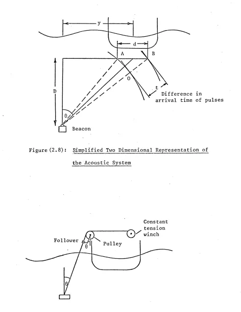
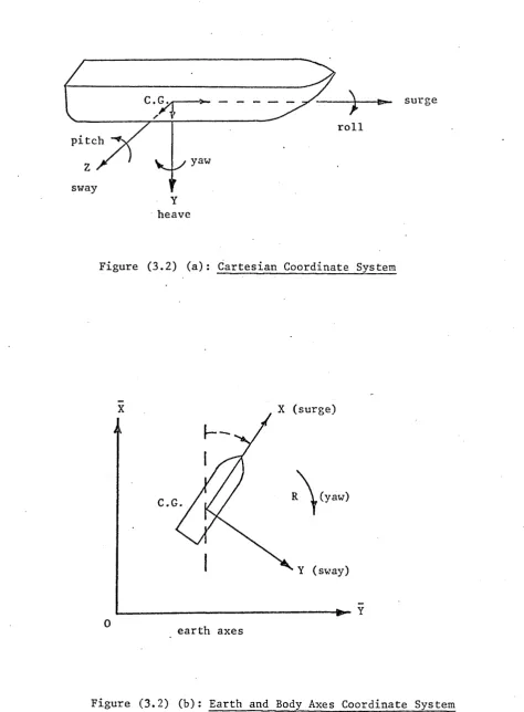
Due to the demand for accuracy within the dynamic positioning systems, the most commonly used technique for measuring the position (Figure 2.8) is based on an acoustic system where a beacon is deployed on the seabed and designed to transmit signals at a frequency around 20 KHz

jjL5] at specific time intervals. The pulses transmitted by the beacon are received at an array of hydrophones fitted at the hull underneath the vessel, and the position of the vessel relative to the beacon is

Difference in

arrival time of pulses

Beacon

Figure (2.8): Simplified Two Dimensional Representation of

the Acoustic System

Constant tension winch

Follower _Pulley

position calculations are carried out by the on-board computer on the

basis of the following formula:

_ -l vfits Dvdt

y = D tan (sm — ^— (2.6)

where:

y the displacement of the vessel

<St the difference in the time of arrival of the pulses

at two of the hydrophones set

v the velocity of sound in water

D the water depth

d the separation between the two hydrophones

The great disadvantage with this technique in providing position reference deviations are the sensitivity to acoustic noise and air

bubbles in the signal transmission line Q.6). In addition to the accuracy requirement of the measurements, reliability and repeatability are also

required. With the hydroacoustic system in operation alone, blocking of measurements in 20-40 per cent of the operation time may occur. To avoid the loss of the measurement signal, and to improve the

reliability of the measurement systems, various back up systems can be used. The most commonly used system is the taut wire system shown in

Figure 2.9, which consists of a sinker weight, wire, tensioning winch and inclinometer. The wire is maintained in tension by means of the constant-tension winch, which is also used to raise and lower the sinker?: weight when required. The measurement inaccuracy within the taut wire

system may arise from the effect of the sea currents and the catenary effect on the wire due to its weight. Measurement systemsdeveloped by

GEC and installed on "Wimpey Sealab" are to consist of one beacon and

taut wire measuring system shown in Figure 2.10. The vessel heading measurements are obtained-by the ship gyro compass.

As to the applications of dynamic ship positioning, considered in this

work, the vessel position accuracy is about ±3 per cent of the water depth of 200 metres and ±2 per cent in 500 metres of water depth. The vessel positional accuracy can be defined by the following expression:

Radial Error = ei.d + W/2 + ez •... (2.7)

where:

e2 is the per unit error of the position measurement system

d is the water depth

W is the peak to peak wave motion e2 is the accuracy of the control loop

2.4 Process and Measurement Noise Analysis

The vessel motions under dynamic positioning control are assumed to consist of low and high frequency components. Our main concern in this section is the low-frequency part of the motions, which are

assumed to be due to the current, wind and the second order wave

forces (Section 3.2). The mean wind forcing level and the sea current

speed and direction are all normally assumed constant over a period of time and up to several hours [74] . Like all environmental phenomena, wind has a stochastic nature which greatly depends on time and location.

To compensate for such uncertain forces, the low-frequency part of the system dynamic is excited by random variables. These random variables are modelled as stationary zero mean and Gaussian white noise sequences.

Mathematically, this means that the probability distribution and

density functions are unchanged over some specific period of time.

The wind forces are often the most important disturbance acting on the vessel. Wind feedforward control is often used to counteract the effect of steady wind (Figure 1.1) and hence, it will be assumed that the vessel positioning will be affected by a white component of wind only. The noise analysis can be extended to include the study of both process and observation noise, which in turn affect the system

estimation for them causing the plant uncertainties.

2.4.1 The Process Noise

The process noise will be considered here in terms of their covariance

matrices. The continuous or discrete time noise covariance matrices are related by the step length of the system simulations time interval

(At), and hence the discrete process covariance matrix will be:

Q - —_{D At (2.8)}

where At is the step length time interval =0.1 and QD is the discrete form of Q. The process covariance matrix (Q) is assumed to consist of a Q submatrix corresponding to the low-frequency part of the system

£

dynamics, and a submatrix corresponding to the high-frequency part of the dynamics.

The high-frequency submatrix in Q is determined by the least squares

fitting procedure [34~] and assumed to be unity (i.e. = I).

The low-frequency part of the system dynamics has a matrix

Hence, per-unit sway force = 126.8/55620 = 0.00228, and per-unit yaw torque = 1636/(55620 x 94.5) = 0.00031. Thus, for two degrees of

freedom in sway and yaw, the low-frequency part of Q-matrix will be:

(0.00228)2 0.0

0.0 (0.00031)

2.4.2 The Observation Noise

The observation or measurement noise and their related covariances will be examined here. The position measuring systems are always

contaminated by superimposed noise and assumed to have a standard

deviation cr = V 3 metre. The per-unit position measurement noise covariance (Appendix 1) therefore will become:

o' (sway) = 0.0033 and (cf)2 = 0.1 x lO-4

The yaw angle standard deviation is assumed to be one degree, and

hence

CHAPTER 3

THE SHIP MOTION

3.1 Introduction

The motion of a ship induced by the waves is an oscillatory motion with frequencies equal to the wave frequencies [l8]. At the same time the

ship drifts off from its original position in the wave direction. Drift of the ship is also induced by the external environmental

forces of wind and current. The current speed and direction may be

constant over some period of time. Current speed and direction changes could occur but these changes are slow compared with fluctuations of wind speed and direction. The wind may be treated as a random Gaussian process (white Gaussian noise throughout the modelling and simulation). The ship motion is also induced by the wave forces which consist of a small drift second-order component and a very large first-order oscillatory component.

Depending on the type of the external acting forces the ship motion [3] is assumed to consist of a low-frequency component and a high-frequency component. The combined motion of the vessel due to both low and high

frequency components [12] is indicated in Figure 3.1. The low-frequency motion in the range of 0.0 - 0.04 Hz (which is 0.0 - 0.251 rad/sec) is assumed to be induced by:

(i) forces generated by the thrusters and propellers,

(ii) hydrodynamic and interaction forces due to the ship motion relative to the water [25] ,

(iii) wind forces,

iw o_{I *H} X U_{00 O}

a •H X_CO a) 4J I_OW CO •U c<u eo a. eo

u

co *H_4J o

£ <a

rd_H

co <u

u

P

00

•H £4

The low-frequency motion will be the combination of the applied forces due to the thrust devices and due to the wind and waves. So that for one degree of freedom:

Total force = f + f, _{a b} (3.1)

where:

f represents the applied forces due to (i), (iii) and (iv) above, f^ represents the hydrodynamic forces in (ii) above.

The high-frequency motions in the range 0.05 - 0.25 Hz (equivalent to 0.314 - 1.57 rad/sec depending on the actual sea spectrum) are assumed to be due to the first-order wave motions. These motions are of a very large level and cause the oscillatory motions of the vessel. These motions cannot be effectively counteracted because of the limited thrust

of the propulsors. The basic assumption for the development of models of the vessel to correspond to the high-frequency motion is that the sea state is known and can be described by a spectral density function. The high-frequency wave motions are normally modelled using the

Pierson-Moskowitz sea spectrum [*5l] .

In the worst case the vessel motions are simply the Pierson-Moskowitz

excitation since the vessel dynamics filter the sea wave spectrum.

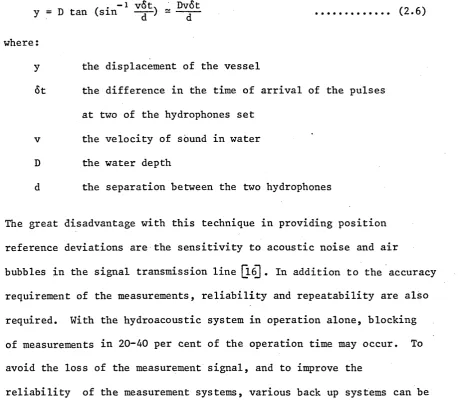
In dynamic positioning^only the vessel motions in the horizontal plane (surge, sway and yaw) are controlled. Heave, roll and pitch motions (Figure 3.2a) are neglected. All motions will be referred to the body

axes of the vessel (Figure 3.2b).

C.G

roll pitch

sway

Y

surge

heave

Figure (3.2) (a): Cartesian Coordinate System

X A

X (surge)

C.

Y (sway)

Y

0 _{earth axes}

motions of the water in the wave [73]. There is differential static

pressure on the hull because of the shape and the gyroscopic couple due to the imposition of rolling motion on the pitching ship. Sway and yaw motions are normally associated with each other. To simplify the

situation, the equations of motion of the vessel in sway and yaw only will be considered. This is possible because the linearised equations of motion indicate that surge motion can be assumed decoupled from the

sway and yaw motions, and hence it can be considered and controlled separately #

3.2 Low-Frequency Dynamics 3.2.1 Introduction

A study of the dynamic positioning control of a vessel at sea requires the formulation of a set of equations which describe its dynamic

behaviour under the forces imposed on it by the environment of wind, waves and current flow as well as by its own thrust producing devices

[l04][7].These equations of motion which represent the vessel dynamics

are assumed to involve a complex multiplicity of coefficients for reasonable accuracy and good modelling to be achieved. Such equations will be regarded as the basis of the whole modelling and simulation

involving the position control scheme of the vessel. However, the need is apparent for a simplification of the set of equations which give a

more realistic feel of the vessel dynamics.

For an efficient control scheme using Kalman filtering, a good

mathematical model of the vessel dynamic is required. The reason for

this is that the Kalman filter uses the model dynamics, together with some knowledge of the noise statistics, to generate the unbiased

estimates of the system states. This assumption will introduce the need

and at the same time provide reasonable representation, good accuracy and simplicity.

The low-frequency part of the vessel dynamics should describe: (i) the wind and wave forces,

(ii) the part of the vessel dynamic to be controlled,

(iii) the thruster dynamics, and

(iv) the interaction between the thrusters devices and the vessel

dynamics.

The dynamic ship positioning system controls the low-frequency part of

the ship motion in surge, sway and yaw. Treating the ship as a rigid body [l04j having freedom of movement in surge, sway and yaw, but restricted in heave, pitch and roll. These movements are taken with

respect to the body axes (Figure 3.2b). The vessel dynamics are represented by a set of non-linear differential equations, then

linearisation procedure has to be applied to these equations for control purpose. The linearised form of the ship equations have the following differential state equation form:

2£o A/ ^2.-2 + ^2— 2 + ^2.-2 + ^2— 2 yv A/ A/ A/ A/ A/ A / A / (3.2)

where:

9

x^(t) £ R are the system state vectors

u^(t) £ R3 are the control inputs to the thrusters

w^(t) £ R 3 are white noise signals representing the random forces applied to the vessel

n^(t) £ R 3 are the wind disturbance forces is the system matrix

is the input matrix

Different parameters and coefficients of equation (3.2) above have been

obtained from a set of tank and wind tunnel tests, carried out by the National Physical Laboratory on two different models, namely "Wimpey

Sealab" and "Star Hercules". The obtained non-linear set of equations have to be linearised, time-scaled and converted into per-unit form, before it can be used in the control loop. Originally, these dynamic equations were provided by GEC Electrical Projects Limited, Rugby, and derived from first principles of Newtonfs laws of motion.

3.2.2 Derivation of the Low-Frequency Dynamics

The body axes are chosen to be the principle axes of the vessel for the derivation of the dynamic equations with its origin located at the centre of gravity (Figure 3.2b). For the position control of a vessel, interest is directly concerned with the motions in the horizontal plane of surge, sway and yaw (Figure 3.2a).

Regarding the vessel as a rigid body having freedom in surge, sway and yaw, but restricted in heave, roll and pitch, the equations of motion

can simply be represented by [iOA] ;

X = m(u - rv) (3.3)

Y = m(v + ru) (3.4)

N = Izzi (3.5)

The forces and moment acting on the vessel in equations (3.3) to (3.5), X, Y and N respectively can be considered as a sum of two components as shown in the following equations:

XA + XH = “ rv) (3.6)

YA + Yr = m(v + ru) (3.7)

where XA , YA and NA represent the applied forces and moment due to the thrust-producing devices, and to the environment of wind and second-order wave drifts.

XH , y h and Nh represent the hydrodynamic forces and moment due to

relative motion between the vessel and the water. To determine the

equations of motion, expressions for Xjj, Yg and Njj are required,

appropriate to a vessel making small movements about a fixed reference position.

Xfl, Yjj and Njj are assumed to be a function of the velocities and

accelerations (u, v, r, u, v and r). It is assumed that the velocity and acceleration dependent forces can be separated. Acceleration dependent forces, referred to as added masses and added iiiertia are X^, Y^ and N^, which depend on the nature of the body motion and flow pattern.

m : mass of the vessel.

I : radius of gyration.

The above equations in (3.6) to (3.8) can now be written as:

XA + x£ ^ “ Y^rv + xH («*v,r)‘ = m(u - rv) (3.9)

YA + Yv * + V U + V u’v ’r> = + ru> ■ •••.... (3*10>

Na + Nf r + NR (u,v,r) = I ^ r (3.11)

Equations (3.9) to (3.11) can be rearranged into the following form:

(m - Xfi)u - (m - Y^)rv = XA + X ^ u ^ r ) (3.12)

(m - Y^)v + (m - X^)ru = YA + YR (u,v,r) (3.13)

(Izz ~ V * = NA + NH (u’v ’r) (3'14)

consideration. The per-unit variables are shown by using a primed symbol, and are obtained using the following base units:

u = _ _ _ , v = , r « —

•^ppg *%pS > V Lpp

.v u .s v r

u = — , v = — , r = — 7-—

g g g/Lpp

£ = — , Y ' = — , IT = — ^—

mg mg mg pp

K-t ^zz

pp-t = ■■-■■■■ ■ , K _

zz Lpp

I . = m'(K')2 = (K' )2_{zz z^ zz}

where:

Lpp is the length between the perpendiculars

g is the gravitational acceleration (= 9.81 m/sec2) K is the radius of gyration in yaw (= 0.243)_zz

The above per-unit system formulas are valid for a vessel with small fixed displacement, which is the case of the dynamic positioning problem.

ii it

3.2.3 Low-Frequency Equations for Wimpey Sealab Vessel

There are a variety of methods by which an estimation of the different coefficients in equations (3.12) to (3.14) can be achievedl These methods are mainly based on experimental results on a model of the

vessel in tank tests, or on a theoretical basis using previous

experimental evidence. An estimation of the coefficients for the drill ship "Wimpey Sealab" is obtained by a combination of results from tank tests and theory, performed at the National Ph}rsical Laboratory [l04j. After reference to the base unit details of "Wimpey Sealab" in Appendix

(1 + 0.044)us - (1 + 0.84)r'vv = + 0.092(v')2

- 0.138iTlf (3.15)

(1 + 0.84)v" + (1 + 0.044)r"uv = - 2.58v"lT

- 1 . 8 4 ( 0 3/lT +0.068r"|r"| (3.16)

((Kk_ZZ )2 + 0.0431)rv = _ii- 0.764u"v" + 0.258vKUv

- 0.162r"|r"| (3.17)

where:

UK = modulus of the vessel velocity (surge and sway) = /(uK)2 + (v)2. The prime is used to denote the per-unit variable. Equations (3.15) to

(3.17) above represent the vessel motions in surge, sway and yaw with

respect to the vessel axes.

For the dynamic ship positioning system, the vessel deviations from its reference position are assumed relatively small, and hence a reasonable

linearisation process can be applied to get a form of linear state equations for simulation and control. Previous experience with Notch filter designs [5l],[99] suggests that a linear low-frequency model

can be good enough for the design and control of the dynamic ship positioning system using a Kalman filtering scheme. The linear state

equations can be obtained using Taylor expansions [65] and some useful approximation to the non-linear dynamics [l04]. However, a number of linearised models could be obtained for different sea current and state of environment. The following linearised dynamics have been used which correspond to a Beaufort number 8 sea state with a mean wind velocity of 19 m/sec:

1.044u*‘ = - 0.01593uv (3.18)

1.84vK = - 0.1004v*' + 0.002981r% (3.19)

As a result of the little interaction between the surge and the sway

and yaw motions within the above equations, simulation and control will be applied initially using the sway and yaw motions only and described by equations (3.19) and (3.20). Surge motion then can be simulated separately.

The low-frequency model for sway and yaw motions is to include the velocity, position and heading of the sway and yaw, as well as to represent the thruster dynamics. The thrusters have been modelled by

simple first order lag terms with two seconds time constant real

time. Referring to Section 2.2, Section 2.4 and Figure 3.3, the overall low-frequency dynamics for "Wimpey Sealab" can be represented by the following state space equation and its related details:

-Z = AZ-Z + BZ-Z + B9^Z + E£nit (3.21)

where:

2£^(t) £ R6 is the system state vectors in. which, xi (t) = sway velocity

X2 (t) = sway position X 3 (t) = angular velocity

(t) = yaw heading

xs (t), X6(t) = thruster outputs u^(t) £ R2 are the control inputs

eim + e2n2 wind disturbance

46

With:

h

T D* ■

e t =

a n 0.0 a l 3 0.0 _{V .} Y23x“ ~0.0 0.0 ~

1.0 0.0 0.0 0.0 0.0 0.0 0.0 0.0

a 3 1 0.0 a 3 3 0.0 Y 332 0.0 0.0

0.0 0.0 1.0 0.0 0.0 0.0 0.0 0.0

0.0 0.0 0.0 0.0 -b! 0.0 bi 0.0

__0.0 0.0 0.0 0.0 0.0 _{-b2 -} _ 0.0 b2

0.0 0.0 0.0 0.0 0.0

_0.0 0.0 _$2 0.0 0.0 0.0

ei3i 0.0 _e3$2 0.0 0.0 0.0

- e2^1 0.0 0.0 0.0 0.0

The low-frequency components of the position and heading is given by:

To = -U ₌ CsAl (3.22)

where:

0.0 1.0 0.0 0.0 0.0 0.0

0.0 0.0 0.0 1.0 0.0 0.0

Substituting for the above different variables in terms of the respective

approximated and calculated values, the following system matrices can be obtained:

Ai

0.0546 0.0 0.0016 0.0 0.5435 0.272

1.0 0.0 0.0 0.0 0.0 0.0

0.0573 0.0 -0.0695 0.0 3.268 -1.634

0.0 0.0 1.0 0.0 0.0 0.0

0.0 0.0 0.0 0.0 -1.55 0.0

0.0 0.0 0.0 0.0 0.0 -1.55