Marra, G. and Radice, Rosalba and Bärnighausen, T. and Wood, S. and
McGovern, M. (2016) A simultaneous equation approach to estimating HIV
prevalence with non-ignorable missing responses. Journal of the American
Statistical Association 112 (518), pp. 484-496. ISSN 0162-1459.
Downloaded from:
Usage Guidelines:
Please refer to usage guidelines at or alternatively
Prevalence with Non-Ignorable Missing Responses
∗
Giampiero Marra
†Rosalba Radice
‡Till Bärnighausen
§Simon N. Wood
¶Mark E. McGovern
kAbstract
Estimates of HIV prevalence are important for policy in order to establish the health status
of a country’s population and to evaluate the effectiveness of population-based interventions
and campaigns. However, participation rates in testing for surveillance conducted as part of
household surveys, on which many of these estimates are based, can be low. HIV positive
in-dividuals may be less likely to participate because they fear disclosure, in which case estimates
obtained using conventional approaches to deal with missing data, such as imputation-based
methods, will be biased. We develop a Heckman-type simultaneous equation approach which
accounts for non-ignorable selection, but unlike previous implementations, allows for spatial
dependence and does not impose a homogeneous selection process on all respondents. In
ad-dition, our framework addresses the issue of separation, where for instance some factors are
severely unbalanced and highly predictive of the response, which would ordinarily prevent
model convergence. Estimation is carried out within a penalized likelihood framework where
smoothing is achieved using a parametrization of the smoothing criterion which makes
esti-mation more stable and efficient. We provide the software for straightforward implementation
of the proposed approach, and apply our methodology to estimating national and sub-national
HIV prevalence in Swaziland, Zimbabwe and Zambia.
Key Words: Heckman-Type Selection Model, HIV, Penalized Regression Spline, Selection
Bias, Simultaneous Equation Model, Spatial Dependence.
∗E-mail for correspondence:[email protected].
†Department of Statistical Science, University College London, Gower Street, London WC1E 6BT, UK.
‡Department of Economics, Mathematics and Statistics, Birkbeck, University of London, Malet Street, London WC1E 7HX, UK.
§
Department of Global Health and Population, Harvard T.H. Chan School of Public Health, Boston, MA, USA. Wellcome Trust Africa Centre for Population Health, University of KwaZulu-Natal, Mtubatuba, South Africa.
1
Missing data in HIV research
Interventions targeted to control the HIV epidemic, improve population health, and reduce HIV-related health disparities, are often motivated by prevalence data obtained from HIV testing (Beyrer et al., 1999; De Cock et al., 2006). In many countries, estimates of HIV prevalence obtained from home-based testing during nationally representative household surveys are now considered the gold stan-dard (Boerma et al., 2003). However, these data can be affected by non-participation because some of those who are eligible opt out of HIV testing. In general, the treatment of missing information in survey data has the potential to have a substantial impact on both the model’s parameter esti-mates and the resulting policy recommendations (Nicoletti, 2006). Because we cannot observe the true outcome for those who do not participate, and because of the role these data have in inform-ing policy, modelinform-ing non-participation in testinform-ing and developinform-ing a framework for accountinform-ing for missing data in a manner which imposes as few assumptions as possible is particularly relevant for the field of HIV research.
Non-participation can occur through a variety of mechanisms, including directly declining to test for HIV when a respondent is approached to test after their interview, or being an eligible respondent for HIV testing but not being present when the interviewers seek to contact the person for interview (Marston et al., 2008). This means that ex post the surveyed group who consent to HIV testing may not be representative of the population of interest. Selection bias occurs if HIV prevalence among those who participate in testing differs from those who do not. In many contexts the extent of non-participation is substantial; for example, 37% of eligible male respondents failed to participate in testing in the 2004 Malawi Demographic and Health Survey (Hogan et al., 2012).
(con-ditional on observed characteristics), then the assumption of missing at random is violated and hence conventional methods, including imputation or analysis based only on non-missing observa-tions, will generate biased results (e.g., Heckman, 1990; Puhani, 2000; Vella, 1998; Janssens et al., 2014). In addition, because imputation-based models do not acknowledge that there is uncer-tainty surrounding the relationship between participation in testing and HIV status, confidence intervals based on this approach are likely to be too narrow when non-participation is common (Hogan et al., 2012).
1.1
Towards a more flexible framework for estimating HIV prevalence
Although the simultaneous equation modeling approach, such as that proposed by Heckman (1979), has the advantage of not requiring the assumption of missing at random, previous techniques im-plementing this model are limited by a number of methodological drawbacks. This article makes four methodological contributions to the literature, and for each of these we outline the relevant problem and illustrate how our framework is designed to correct for the issue.
that could be done with previous implementations is to stratify according to the group of interest, however given the resulting inefficiency and that sample sizes can be low across groups, this is not a realistic solution. Our proposal has potentially important applications beyond HIV research and will likely be of interest in situations in which there is spatial dependence and missing data.
Second, we extend the selection framework to allow for the utilization of ridge penalties to deal with problematic parameters (associated with categorical regressors, for instance) which would ordinarily lead to convergence failure. It is known that, with binary responses the problem of separation, where for instance some factor variables are severely unbalanced and highly predictive of the response, often prevents algorithms from converging (e.g., Heinze & Schemper, 2002). In practice, the bivariate probit models which have been used to implement selection models when the outcome is binary are not very stable and fail to converge relatively frequently (Butler, 1996; Clark & Houle, 2014). Therefore, there is a danger that such models are only employed in cases with specific data configurations. In our case study, we apply a ridge penalty on the parameters of the selection variable, interviewer identity. As we describe further in the next section, the selection variable can be thought of as an instrumental variable in that it predicts participation but is assumed not to predict directly the outcome of interest (Madden, 2008). In all three countries considered in our analysis, we were unable to implement the traditional selection model. The interviewers in these surveys are often matched to participants on the basis of some group-level characteris-tics (e.g., language). Moreover, some interviewers obtain participation in testing from all their interviewees, while for some other interviewers all their interviewees may decline to participate. This means that some interviewer effects will not be estimable due to lack of within-interviewer variation in testing participation. Solutions involving pooling very successful interviewers with very unsuccessful interviewers, dropping problematic interviewers, or estimating interviewer per-suasiveness in a two-stage process are clearly not desirable (McGovern et al., 2015a). To the best of our knowledge, there is no alternative implementation of selection models which would allow us to deal with the above mentioned issue in a theoretically founded way. Given that, in practical applications, selection models often suffers from these types of convergence failures, it is likely that our proposed development will be of use beyond the HIV study considered in this article.
Radice et al., 2015). This has the advantage of making smoothing parameter estimation more stable and efficient. Our derivations also show that the proposed approach can in principle be applied to any situation in which a model is fitted by penalized maximum likelihood, thereby appealing to a wider audience of researchers.
Fourth, all the developments discussed in this article have been made available through the freely distributed and easy to use R package SemiParBIVProbit (Marra & Radice, 2016), which can allow researchers and policy-makers to apply a flexible selection approach to account for systematic non-participation in their data.
Our methodology incorporates each of these developments in a flexible simultaneous equation framework for adjusting for systematic non-participation in HIV surveys. We outline further de-tails of this methodology in the rest of the paper as follows. Section 2 introduces the approach in more detail by describing its main statistical components, including estimation and inference. Sections 3 and 4 describe the data and apply the proposed approach to three Sub-Saharan African countries (Swaziland, Zambia, and Zimbabwe). In Section 5, we outline two approaches for eval-uating the sensitivity of results to model assumptions. The final section provides a discussion and directions for future research.
2
Extending Heckman-type selection models
the reliance on the assumption of bivariate normality and the lack of flexibility in modeling co-variate effects. Subsequent developments have addressed these issues (Marra & Radice, 2013; McGovern et al., 2015b) and have represented the starting point for our proposed extensions.
Selection models require a valid instrument for identification. As mentioned in the previous section, interviewer identity will serve as an exclusion restriction in our study. The identity of the interviewer who contacts the respondent to seek consent for an HIV test is often recorded in survey data as an anonymized code. The allocation of interviewers to eligible survey respondents is typically highly correlated with whether the respondents consent to test. Such allocation is also based on survey design features, as opposed to the characteristics of the respondents themselves. Therefore, interviewer identity is plausibly exogenous and should be unrelated to the HIV status of survey respondents. In other words, interviewer identity satisfies potentially the condition of exclusion restriction (Bärnighausen et al., 2011). The validity of this assumption is discussed further in Section 5.2.
2.1
Model representation
Let us assume that there are two random variables (Y1i, Y2i), for i = 1, . . . , n, where Y1i, Y2i ∈
{0,1} and n represents the sample size. Variable Y1i indicates whether an individual takes part
in the study whereas Y2i denotes the outcome. The probability of event (Y1i = 1, Y2i = 1),
conditional on the sets of covariates z1i and z2i, can be defined as (Kolev & Paiva, 2009; Sklar,
1959, 1973; Zimmer & Trivedi, 2006)
p11i =P(Y1i = 1, Y2i = 1|z1i,z2i) =C(P(Y1i = 1|z1i),P(Y2i = 1|z2i);θi),
whereP(Yvi = 1|zvi) = Φ(ηvi)forv = 1,2,Φ(·)is the cumulative distribution function (cdf) of
the standard univariate Gaussian distribution,ηvi ∈ Ris a linear predictor made up of regression
coefficients and covariates (defined in generic terms in the next section),C is a two-place copula function and θi is an association parameter measuring the dependence between the two random
variables. Since the strength of the association between the selection and outcome equations may vary across groups of observations (specifically, across regions in our case), in our framework we allow the copula dependence parameter to be specified as a function of a linear predictor. That is,
lies in its range, and η3i is the linear predictor associated with the copula parameter. For the
list of transformations and copulae (as well as the counter-clockwise rotated versions of some of them) see Radice et al. (2015). In this context, Y2i is available only ifY1i = 1, hence the only
additional events are(Y1i = 1, Y2i = 0)and(Y1i = 0), with probabilitiesp10i = Φ(η1i)−p11i and
p0i = Φ(−η1i). Therefore, the log-likelihood function of the sample is expressed as
ℓ=
n
X
i=1
{y1iy2ilog(p11i) +y1i(1−y2i) log(p10i) + (1−y1i) log(p0i)},
wherey1i andy2iare realizations ofY1iandY2i, respectively.
2.2
Linear predictor specification
For simplicity, and without loss of generality, we suppress subscriptvand define the generic linear predictor as
ηi =β0 + K
X
k=1
sk(zki), i= 1, . . . , n, (1)
where β0 ∈ R is an overall intercept, zki denotes the kth sub-vector of the complete
covari-ate vectorzi (which contains, e.g., binary, categorical, continuous and spatial variables), and the
K functionssk(zki) represent generic effects which are chosen according to the type of
covari-ate(s) considered. Eachsk(zki)can be approximated as a linear combination ofJk basis functions
bkjk(zki)and regression coefficientsβkjk ∈R, i.e.
Jk
X
jk=1
βkjkbkjk(zki). (2)
Equation (2) implies that the vector of evaluations{sk(zk1), . . . , sk(zkn)}Tcan be written asZkβk,
with coefficient vectorβk= (βk1, . . . , βkJk)
Tand design matrixZ
k[i, jk] =bkjk(zki). This allows
us to write the linear predictor in equation (1) as
η=β01n+Z1β1+. . .+ZKβK, (3)
where1nis ann-dimensional vector made up of ones. Equation (3) can also be written in a more
compact way asη =Zβ, whereZ = (1n,Z1, . . . ,ZK)andβ = (β0,βT1, . . . ,βTK)T. The smooth
functions may represent linear, non-linear, random and spatial effects, to name but a few. More-over, each βk has an associated quadratic penalty λkβkTDkβk whose role is to enforce specific
properties on thekth function, such as smoothness. D
k is defined in the next paragraphs for
and plays a crucial role in determining the shape of sˆk(zki); a large value for λk means that the
corresponding penalty has a large influence on the parameters of the function during fitting, and viceversa. The overall penalty can be defined asβTD
λβ, whereDλ= diag(0, λ1D1, . . . , λKDK).
Note also that smooth functions are subject to centering (identifiability) constraints and we em-ploy the parsimonious approach detailed in Wood (2006) to deal with this issue. In the following paragraphs, we outline the rationale for adopting the specific model components relevant to our case study.
Spatial effects To model the spatial information based on the geographic location of survey
respondents, we employ a Markov random field smoother. This approach is popular when the geographic area (or country) of interest is split up into discrete contiguous geographic units (or regions), and allows us to take advantage of the information contained in neighboring observations which are located in the same country. In this case, equation (2) becomes zTkiβk, where βk =
(βk1, . . . , βkR)T represents the vector of spatial effects, R denotes the total number of regions,
and zki is made up of a set of area labels. The design matrix linking an observation i to the
corresponding spatial effect is therefore defined as
Zk[i, r] =
1 if the observation belongs to regionr
0 otherwise
,
wherer = 1, . . . , R. The smoothing penalty is based on the neighborhood structure of the geo-graphic units, so that spatially adjacent regions share similar effects. That is
Dk[r, q] =
−1 ifr6=q∧ randqare adjacent neighbors
0 ifr6=q∧ randqare not adjacent neighbors
Nr ifr=q
,
whereNr is the total number of neighbors for regionr. In a stochastic interpretation, this penalty
is equivalent to the assumption thatβkfollows a Gaussian Markov random field (e.g., Rue & Held,
Linear and random effects For parametric, linear effects, equation (2) becomeszT
kiβk, and the
design matrix is obtained by stacking all covariate vectorszki intoZk. In general, no penalty is
assigned to linear effects(Dk = 0). This would be the case for variables such as ever tested for
HIV and condom use at last sexual activity. However, sometimes the parameters of factor variables such as interviewer identity may be weakly or not identified by the data (see Section 1.1). In such cases, we recommend using a ridge penalty (i.e.,Dk = I, whereIis an identity matrix) to make
the model parameters estimable. This is equivalent to the assumption that the coefficients arei.i.d.
normal random effects with unknown variance (e.g., Ruppert et al., 2003; Wood, 2006).
Non-linear effects For continuous variables such as age and years of education the smooth
func-tions are represented using the regression spline approach popularized by Eilers & Marx (1996). Specifically, for each continuous variablezki we use equation (2), where thebkjk(zki)are known
spline basis functions. The design matrixZk comprises the basis function evaluations for eachi,
and describe theJk curves which have varying degrees of complexity. We employ low rank thin
plate regression splines (Wood, 2003) which are numerically stable and have convenient math-ematical properties, although other spline definitions (including B-splines and cubic regression splines) and corresponding penalties are supported in our implementation. To enforce smoothness, a conventional integrated square second derivative spline penalty is typically employed. That is,
Dk =
R
dk(zk)dk(zk)Tdzk, where thejkth element ofdk(zk)is given by∂2bkjk(zk)/∂z
2
k and
inte-gration is over the range ofzk. The formulae used to compute the basis functions and penalties
for many spline definitions are provided in Ruppert et al. (2003) and Wood (2006). This flexible spline approach allows us to avoid arbitrary modeling decisions, such as choosing the appropriate degree of a polynomial or specifying cut-points, which could induce misspecification.
In the context of our study, the linear predictors for the selection (η1) and outcome equations (η2)
and for the copula parameter (η3) are specified as
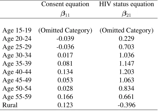
η1i =β10+xTi β11+s11(agei) +s12(educationi) +s13(wealthi) +s1spatial(regioni) +βinterviewerIDi,
η2i =β20+xTi β21+s21(agei) +s22(educationi) +s23(wealthi) +s2spatial(regioni),
η3i =β30+s3spatial(regioni),
where parametersβ10,β20,β30are constants comprising the overall levels of the predictors, vector
equa-tions, β11 andβ21 are the respective parameter vectors, thesvk forv = 1,2andk = 1,2,3 are
smooth functions of age, education and wealth represented using penalized thin plate regression splines, and thesvspatialforv = 1,2,3model spatial regional effects using a Markov random field
approach. Finally,βinterviewerIDi denotes the random effects for the set of binary variables defined
by interviewer identity. The variables included inxi are: type of location (urban or rural),
mari-tal status, had a sexually transmitted disease, age at first intercourse, had high risk sex, number of partners, condom use, would care for an HIV-infected relative, knows someone who died of AIDS, previously tested for HIV, smokes, drinks alcohol, language, region, ethnicity and religion. The choice of variables followed previous studies which examined the predictors of testing and HIV status in detail (Bärnighausen et al., 2011; Hogan et al., 2012). Linear predictor η3 models the
presence of unobserved confounders and therefore specifying the predictor equation as a function of observed characteristics only makes sense from an estimation perspective if there are groups for which there is a clear rationale for expecting heterogeneity in the selection process. While in theory we could include additional group-level identifier variables, we opt to specify the cop-ula parameter as depending on region. This parametrization is motivated by the evidence on the spatial clustering of HIV prevalence (Larmarange & Bendaud, 2014; Tanser et al., 2009). There are other types of smooth functions that could be incorporated in our framework, should they be required. These include varying coefficient models obtained, for instance, by multiplying one or more smooth components by some predictor(s), and smooth functions of two or more continu-ous covariates; see Hastie & Tibshirani (1993), Ruppert et al. (2003) and Wood (2006) for more details.
2.3
Parameter estimation
Let us define the overall quantitiesδT= (βT
1,β2T,β3T)andSλ= diag(λ1D1,λ2D2,λ3D3), where
λT
v = (λvkv, . . . , λvKv)forv = 1,2,3. The parameter vectors and matrices that make upδandSλ
are related toη1i,η2iandη3i. Because of the flexible linear predictor specifications employed here,
the use of a classic (unpenalized) optimization algorithm is likely to result in function estimates that may not reflect the true underlying trends in the data (e.g., Ruppert et al., 2003; Wood, 2006). Therefore, we maximize
ℓp(δ) = ℓ(δ)−
1
2δ
TS
Estimation of δ and λ is carried out in two steps. Given λˆT = (ˆλT
1,λˆT2,λˆT3), we seek to
maximize (4). As in Radice et al. (2015), we use a trust region approach which is generally more stable and faster than its line-search counterparts (such as Newton-Raphson), particularly for functions that are, for example, non-concave and/or exhibit regions that are close to flat (Nocedal & Wright, 2006, Chapter 4). Let us define the penalized gradient and Hessian at iteration
aasg[a]p =g[a]−Sλ[a]δ[a]andH[a]
p =H [a]
−Sλ[a], whereg[a]consists ofg[a]
1 =∂ℓ(δ)/∂β1|β1=β[a]
1 ,
g[a]2 = ∂ℓ(δ)/∂β2|β2=β[a]
2
and g[a]3 = ∂ℓ(δ)/∂β3|β3=β[a]
3
, and the Hessian matrix has elements
H[a]
o,h = ∂2ℓ(δ)/∂βo∂βhT|βo=β[ a] o ,βh=β[
a] h
with o, h = 1, . . . ,3. For a given λ[a], the trust region algorithm solves the problem
min
p
˘
ℓp(δ[a])
def
=−
ℓp(δ[a]) +pTg[a]p +
1
2p
TH[a] p p
such that kpk ≤ra[a],
δ[a+1]= arg min
p
˘
ℓp(δ[a]) +δ[a],
where k · k denotes the Euclidean norm and ra[a] is the radius of the trust region; full details
can be found, e.g., in Geyer (2015). Note that, near the solution, the trust region method typically behaves as a classic unconstrained algorithm (e.g., Nocedal & Wright, 2006). Our implementation provides the possibility of usingE(H[a])instead of the default optionH[a]. However, as in Wood
(2011), we generally found observed information to be superior in terms of speed, stability and accuracy of results (Efron & Hinkley, 1978).
The second step concerns smoothing parameter selection. There are a number of methods for automatically estimating smoothing parameters within a penalized likelihood framework, and in the context of bivariate equation models the approach discussed in Radice et al. (2015) and Marra & Radice (2013) has proven successful. However, for the models considered in this paper such a scheme may be unstable and inefficient when the linear predictors are highly flexible and the copula parameter is specified as a function of covariates (see Supplementary Material (SM)-A for a through explanation of this). We therefore perform smoothing parameter estimation using an alternative (more stable and efficient) parametrization of the smoothing criterion. After some manipulation, the model’s parameter estimator can be expressed as
δ[a+1]=I[a]+Sλ[a]
−1p
I[a]z[a], (5)
whereI[a] =−H[a],z[a] =pI[a]δ[a]+ǫ[a]andǫ[a]=pI[a]−1g[a]. From likelihood theory,ǫ∼ N(0,I)andz∼ N (µz,I), whereIis an identity matrix,µz =
√
vector. The predicted value vector forzisµˆz = √
Iδˆ=Aˆ
λz, whereAλˆ =
√
I(I+Sˆ
λ)
−1√I
. Representation (5) allows us to base smoothing parameter estimation on a parametrization ofzthat usesHandgas a whole instead of thencomponents that make them up. As elaborated in SM-A,
this is advantageous in our context. Since our goal is to estimate λ so that the smooth terms’ complexity which is not supported by the data is suppressed, the smoothing parameter vector is estimated so thatµˆz is as close as possible toµz. Using this, for a givenδ[a+1], the problem to
minimize becomes
λ[a+1]= arg min
λ V
(λ)def= kz[a+1]−A[a+1]λ[a] z
[a+1]k2−nˇ+ 2tr(A[a+1]
λ[a] ),
wherenˇ = 3n, which is solved using the automatic stable and efficient computational routine by Wood (2004). Details on the derivation of the results stated above are provided in SM-A.
2.4
Further considerations
Estimation of λ is achieved using gand I which are obtained as a byproduct of the estimation
step for δ, hence little computational effort is required to set up the quantities needed for the smoothing step. The additional key benefit of usingzandAas defined in the previous section is that the proposed smoothing approach is in principle suitable for any model fitted by penalized maximum likelihood. Consistency of the proposed estimator can be proved along the lines of Wojtys & Marra (2015), but this is beyond the scope of this paper.
At convergence, reliable point-wise confidence intervals for linear and non-linear functions of the model coefficients (e.g., smooth components, prevalence estimates, copula parameter) can be obtained usingN( ˆδ,−Hˆ−1
p ). The rationale for using this result is provided in Marra & Wood
(2012), and references therein, and some examples of interval construction are given in Radice et al. (2015). We can also test smooth components for equality to zero using the results discussed in Wood (2013a) and Wood (2013b). However, we do not deem this necessary as we followed the pre-vious literature for variable selection (Bärnighausen et al., 2011; Hogan et al., 2012). HIV preva-lence estimates are obtained using Pn
i=1wiΦ(ˆη2i)/Pni=1wi, where the wi are survey weights,
while confidence intervals are derived using the delta method or posterior simulation using the above mentioned distributional result (e.g., McGovern et al., 2015b).
For the reader’s convenience, we have summarized the letters and symbols used in the paper and their corresponding meanings in the table reported in the last section of the Supplementary Material (SM-F).
3
Data
We implement the extended simultaneous equation model framework to estimate HIV prevalence in three sub-Saharan African countries. Data are obtained from the Demographic and Health Sur-veys (DHS) conducted in Zambia in 2007, Zimbabwe in 2005-2006, and Swaziland in 2006-2007. For further details on the DHS and HIV testing procedures, see Corsi et al. (2012), Fabic et al. (2012) and Mishra et al. (2006). Regional identifiers for respondents are used in this analysis, along with information on spatial boundaries at the sub-national level from http://gadm.org/. DHS are not designed to be representative below the regional level, and sampling within regions can be sparse. Therefore, in this analysis we focus on regional level heterogeneity in estimating HIV prevalence.
We follow the previous literature by including inxithe variables described at the end of Section
2.2. Unlike the previous literature, we specify smooth functions of age, years of education, and wealth index (based on household assets) and employ Markov random field smoothers to model spatial variation. All these components enter into the linear predictors for participation (η1) and
HIV status (η2). Exclusion restriction is achieved by including interviewer identity intoη1 only.
We apply a ridge penalty to the coefficients of this variable in order to account for the difficulties associated with its use which we outlined in Section 1.1. Linear predictor η3 only depends on
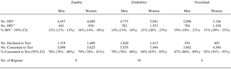
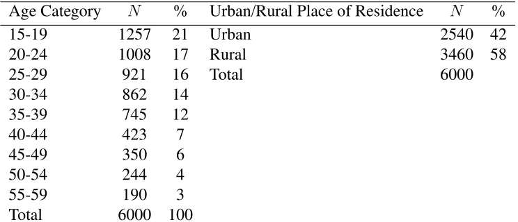
a Markov random field term and allows for the copula association parameter to vary by region. All of our models are stratified by sex to reflect potentially sex-specific consent and HIV related factors. All our prevalence estimates are weighted to be nationally representative. We do not weight during model fitting as the variables on which the DHS weights are based are already included in the model (Hogan et al., 2012). Nevertheless, we have conducted a sensitivity analysis where we use the weights as part of the model fitting procedure and have found very similar results. Table 1 illustrates the sample size, number of regions, number of respondents who participate in testing, and the number of respondents who are HIV positive (among those who participate in testing) in each survey.
eligi-Zambia Zimbabwe Swaziland
Men Women Men Women Men Women
No. HIV− 4,457 4,689 4,773 5,941 2,898 3,146
No. HIV+ 641 936 782 1,553 704 1,438
% HIV+(95% CI) 12% (11% - 13%) 16% (14% - 18%) 14% (13% - 16%) 21% (20% - 23%) 19% (18% - 21%) 31% (29% - 33%)
No. Declined to Test 1,318 1,400 1,620 1,413 554 403
No. Consented to Test 5,098 5,625 5,555 7,494 3,602 4,584
% Consented to Test (95% CI) 78% (76% - 80%) 79% (78% - 81%) 78% (76% - 80%) 84% (83% - 85%) 87% (86% - 89%) 92% (91% - 93%)
[image:15.595.73.534.53.191.2]No. of Regions 9 10 4
Table 1: Descriptive Statistics for Demographic and Health Survey HIV Data. HIV prevalence (%) and consent to test (%) estimates are weighted, and confidence intervals are clustered to account for survey design. HIV status is only available for those who consent to test. Individuals who were eligible but not contacted to test for HIV are not included in the analysis.
ble respondents consenting to test for HIV ranging from 78% for men in Zambia and Zimbabwe, to 92% for women in Swaziland. The percentage of HIV positive individuals (among those who consent to test) is high in all countries, and ranges from 12% for men in Zambia to 31% among women in Swaziland. Confidence intervals for the HIV prevalence estimates which do not account for non-participation are between 3 and 4 percentage points wide in each country.
In this paper, we focus on non-participation due to eligible respondents declining to test for HIV after interview. The amount of missing data due to this type of non-participation is typ-ically more substantial than non-participation due to eligible respondents not being available for interview (Hogan et al., 2012). In addition, previous analysis of the Zambia data found lit-tle evidence of selection bias among this second group (Bärnighausen et al., 2011). The HIV datasets used for the analysis are freely available from http://www.measuredhs.com after registra-tion, and the code for preparing the data can be obtained from http://hdl.handle.net/1902.1/17657 (Bärnighausen et al., 2011; Hogan et al., 2012). In the following section, we present new sex-specific national HIV prevalence point estimates and confidence intervals, and illustrate the re-gional heterogeneity in HIV prevalence and dependence parameter in each country.
4
Results
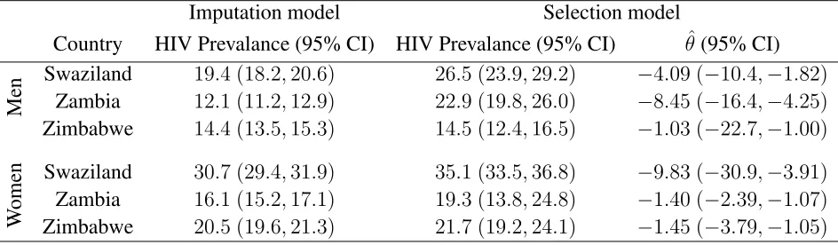
Imputation model Selection model
Country HIV Prevalance (95% CI) HIV Prevalance (95% CI) θˆ(95% CI)
M
en Swaziland 19.4 (18.2,20.6) 26.5 (23.9,29.2) −4.09 (−10.4,−1.82)
Zambia 12.1 (11.2,12.9) 22.9 (19.8,26.0) −8.45 (−16.4,−4.25)
Zimbabwe 14.4 (13.5,15.3) 14.5 (12.4,16.5) −1.03 (−22.7,−1.00)
W
o
m
en Swaziland 30.7 (29.4,31.9) 35.1 (33.5,36.8) −9.83 (−30.9,−3.91)
Zambia 16.1 (15.2,17.1) 19.3 (13.8,24.8) −1.40 (−2.39,−1.07)
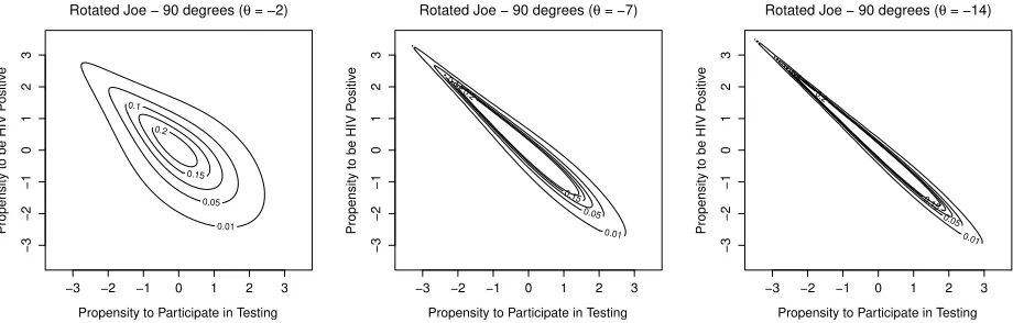
[image:16.595.71.543.52.190.2]Zimbabwe 20.5 (19.6,21.3) 21.7 (19.2,24.1) −1.45 (−3.79,−1.05)
Table 2: National estimates of HIV prevalence (and associated confidence intervals) obtained from the single imputa-tion and proposed simultaneous equaimputa-tion approaches. The estimates shown in column 1 do not account for potentially systematic non-participation whereas those in column 2 do. The dependence structure used for estimating the sample selection models is based on the Joe copula rotated by 90 degrees. Because we specify the dependence parameter in terms of a linear predictor, the values shown in column 3 are the average values in each country. Intervals are calculated using the inferential result mentioned in Section 2.4. The range ofθis(−∞,−1), with higher values (in absolute terms) indicating greater association; Figure 1 in SM-C shows three dependence scenarios.
estimates is that the latter is the recommended approach for dealing with missing data in HIV research by UNAIDS/WHO, and is also very popular in the applied literature for dealing with data affected by missingness. As was found in previous research, imputation estimates are al-most identical to those in Table 1 which were based only on observations without missing data (Mishra et al., 2008; Marston et al., 2008; Hogan et al., 2012; Bärnighausen et al., 2011). More-over, the imputation-based confidence intervals are, similarly, between 3 and 4 percentage points wide. Column 2, which shows our selection model estimates, which account for potentially sys-tematic non-participation, indicate evidence of selection bias for men (Swaziland and Zambia) and women (Swaziland). In each of these cases, we can reject that the selection model point estimates are the same as the imputation-based approach, or analysis of observations without missing data.
In the final column of Table 2, we present estimates of the copula association parameter which measures the degree of association between participation in testing and HIV status (conditional on observed covariates). The values shown in column 3 are the average values in each country. The range of this parameter is(−∞,−1), with higher values (in absolute terms) indicating greater association. Three dependence scenarios for the90◦ rotated Joe copula are illustrated in Figure 1
are close to those of the imputation-based approach. However, even if point estimates are similar, we find that the imputation method substantially understates the amount of uncertainty associated with estimating HIV prevalence when survey testing data are affected by non-participation; con-fidence intervals obtained from the selection model are generally twice as wide as those from the single-equation approach. 5 10 15 20 25 30
HIV (%) − Imputation Model
SW AZILAND Hhohho Lubombo Manzini Shiselweni 5 10 15 20 25 30
HIV (%) − Selection Model
2 4 6 8 10 12 14 Copula Parameter 5 10 15 20 25 30 ZAMBIA Central Copperbelt Eastern Luapula Lusaka North−western Northern Southern Western 5 10 15 20 25 30 2 4 6 8 10 12 14 5 10 15 20 25 30 ZIMBABWE Manicaland Mashonaland central Mashonaland east Mashonaland west Matebeleland north Matebeleland south Midlands Masvingo H B H: Harare
B: Bulawayo 5
[image:17.595.71.539.175.579.2]10 15 20 25 30 2 4 6 8 10 12 14
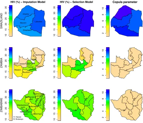
Figure 1: Sub-national HIV prevalence estimates for men obtained by applying the single imputation and proposed simultaneous equation approaches. The copula dependence parameter plot reports the estimated absolute values ofθ
with range(1,∞)in a Joe copula rotated by 90 degrees. The higher the value, the stronger the association between the selection and outcome equations.
We have considered a number of different dependence structures for estimating these models, the majority of which do not rely on the assumption of bivariate normality. Using the Akaike information criterion (AIC), we found that the Joe copula rotated by 90 degrees was the preferred choice for most cases, and therefore all estimates in Table 2 use this dependence structure.
de-pendence parameters, are presented in Figures 1 (men) and 2 (women). There is clear variation in HIV prevalence within some countries, most notably for men in Zambia and women in Zambia and Zimbabwe, either on the basis of the imputation-based model, or the selection model estimates.
10 15 20 25 30 35
HIV (%) − Imputation Model
SW AZILAND Hhohho Lubombo Manzini Shiselweni 10 15 20 25 30 35
HIV (%) − Selection Model
2 4 6 8 10 Copula parameter 10 15 20 25 30 35 ZAMBIA Central Copperbelt Eastern Luapula Lusaka North−western Northern Southern Western 10 15 20 25 30 35 2 4 6 8 10 10 15 20 25 30 35 ZIMBABWE Manicaland Mashonaland central Mashonaland east Mashonaland west Matebeleland north Matebeleland south Midlands Masvingo H B H: Harare
B: Bulawayo 10
[image:18.595.68.540.128.532.2]15 20 25 30 35 2 4 6 8 10
Figure 2: Sub-national HIV prevalence estimates for women obtained by applying the single imputation and proposed simultaneous equation approaches. The copula dependence parameter plot reports the estimated absolute values ofθ
with range(1,∞)in a Joe copula rotated by 90 degrees. The higher the value, the stronger the association between the selection and outcome equations.
For men in Zambia, the selection model HIV prevalence estimates range from28% (24%,32%)
non-overlapping intervals. In Swaziland, which is relatively more homogeneous, the selection model HIV prevalence estimates differ by 6 percentage points between the region with the highest preva-lence (29% (26%,32%)in Hhohho) and lowest prevalence (23% (21%, 26%) in Shiselweni) for men, and 3 percentage points between the region with the highest prevalence (36% (34%,38%)
in Hhohho) and lowest prevalence (33% (31%,35%) in Shiselweni) for women. However, these estimates have overlapping intervals.
There is also support for a heterogeneous selection process across regions within some of these countries, as we find the copula dependence parameter varies according to location. For example, for men in Zambia, the selection model HIV prevalence for Northwestern is 8 percentage points greater than the imputation-based model (13% compared to 5%), while for Luapula, the differ-ence is 9 percentage points (16% to 25%). In addition to this heterogeneity at the regional level, compared to a model which imposed homogeneity on the copula parameter, we found that this approach of allowing the dependence to reflect spatial variation was more efficient for estimating national HIV prevalence.
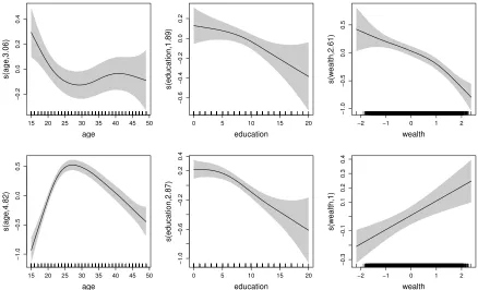
There are important non-linearities and functional form differences across sex and country in the association between observed characteristics of survey respondents and testing participation and HIV status outcomes, which highlights the relevance of our spline and penalized smoothing framework (see SM-E).
5
Sensitivity of results to violations of model assumptions
parametric assumptions and exclusion restriction.
5.1
Simulation study
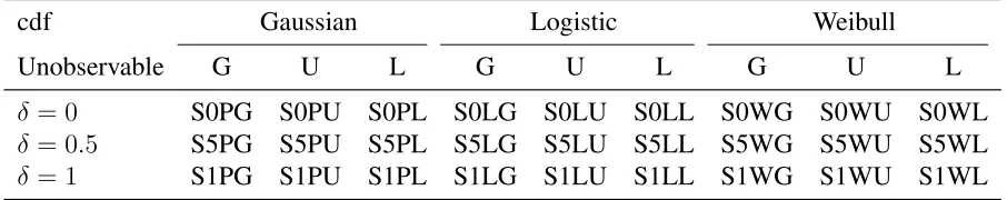
We assess the empirical effectiveness of the proposed sample selection modeling framework through a simulation study, in which we use the results presented in the previous section and employ parsimonious model settings to maintain feasibility. We constructed responses for con-sent and HIV status using several unobserved confounding variable distributions (normal, uniform and log-normal) and link functions (derived from the Gaussian, logistic and Weibull cumulative distribution functions). Imposition of assumptions about the model’s link functions has been a criticism of selection models with continuous response (Kenward, 1998). For each of these nine combinations, we considered the situation in which the exclusion restriction assumption holds (i.e., interviewer identity predicts participation in HIV testing but not HIV status), and the cases where the assumption is mildly and strongly violated. Interest was in prevalence estimates. Exact simulation settings of the resulting 27 scenarios are given in SM-D.
We present results for the best-case and worst-case scenarios (called S0PG, S0WL and S1WL in Table 3 of SM-D). Figure 3 compares the results from the single imputation model, classic Heckman model (assuming bivariate normality) and the preferred copula selection model (as de-termined by the AIC). Figure 3a confirms that, when the Gaussian assumption holds and the exclu-sion restriction is valid, the traditional selection model is appropriate for correcting for systematic non-participation (bias in absolute value = 1.6% and root mean squared error (RMSE) = 0.04) and that the single imputation model performs poorly (bias = 49% and RMSE = 0.107). The wider variability of the selection model estimates as compared to those of single imputation is not surprising; imputation-based models do not acknowledge the uncertainty surrounding the rela-tionship between participation in testing and HIV status. Figure 3b shows the results under model misspecification (Weibull link function and log-normal unobserved confounder) when the exclu-sion restriction holds. The performance of the Gaussian selection model worsens (bias= 19.2%). In contrast, the preferred copula model (in this case the90◦ rotated Joe, although the90◦ rotated
Gumbel and270◦rotated Clayton copulae unsurprisingly produced similar results) gives a bias of
violated) and under model misspecification, the Gaussian and Joe90◦copula selection models
per-form poorly (see Figure 3c), although the latter is less biased and has lower RMSE as compared to the former (bias of 22% and 17% and RMSE of 0.072 and 0.067, respectively).
u g u st (2 0 1 6 ), T o ap p ea r in th e Jo u rn a l o f th e A m er ic a n S ta tis tic a l A ss o ci a tio n 0.10 0.15 0.20 0.25 0.30
Single Imputation Gaussian Selection Model
(a) Scenario S0PG
0.10
0.15
0.20
0.25
0.30
Gaussian Selection Model Copula Selection Model
(b) Scenario S0WL
0.10
0.15
0.20
0.25
0.30
Gaussian Selection Model Copula Selection Model
[image:22.595.77.784.181.364.2](c) Scenario S1WL
Figure 3: Simulation results of prevalence estimates obtained under the best-case (S0PG) and worst-case scenarios (S0WL and S1WL) considered in this paper. In S0PG the unobserved confounder distribution and cumulative distribution function (used to derive the link function) were both Gaussian. In S0WL and S1WL the unobserved confounder distribution and cumuative function were Log-normal and Weibull. In S0PG and S0WL a valid exclusion restriction was employed, whereas in S1WL the assumption that interviewer identity predicts participation in HIV testing but not HIV status was violated. The number of replicates was 250 and the horizontal lines represent the true prevalence. Prevalence estimates were obtained using the single imputation, classic Gaussian selection and preferred copula selection models. Exact simulation settings are given in SM-D.
2
5.2
Plausibility of the exclusion restriction
Since it is generally not possible to empirically test whether an exclusion restriction holds, we provide some arguments as to why interviewer assignment satisfies potentially this assumption. In particular, we explain how interviewers are allocated to respondents in the DHS and use an empirical approach which helps us gain some insights into the plausibility of this assumption.
The sampling procedure for the DHS is designed in two stages. First, a random sample of pri-mary sampling units (PSU) is drawn where geographic locations are usually defined by a preceding census; PSU sampling is often stratified by urban/rural location, and/or region. Then, a random sample of households is chosen within each PSU, and all eligible residents of these households are sought for interview. There are several aspects of the DHS procedure which support the assump-tions that interviewer identity satisfies the exclusion restriction assumption. Two-stage sampling is designed to provide a systematic way of selecting households to participate in the survey, and the DHS procedure recommends that households be pre-selected in the central office rather than by teams in the field. Therefore, the opportunity for interviewers to select who they interview is limited, and interviewer allocation by field supervisors is recommended to be made on the basis of equally distributing workload and linguistic capability (ICF International, 2015). If DHS guide-lines are followed, the risk of bias associated with violation of the exclusion restriction seems low.
anal-ysis where we included the mean characteristics of each interviewer’s interviewees, say ¯xi, as
additional predictors in the HIV status outcome equation. Because we expect interviewers and respondents to be matched on region and language, we could not include these in ¯xi but these
controls remained inxi. Using this empirical approach led to very similar results to those in the
main analysis, hence suggesting that the assumption of exclusion restriction is reasonable.
An alternative way of approaching the validity of the exclusion restriction is provided by Angrist et al. (1996). These authors theoretically derive the bias associated with violation of the exclusion restriction in their application. Due to the complexity of our model, it is not clear how to derive the relevant bias theoretically. However, the simulation results provide us with an indication of the potential consequences for our estimates if the exclusion restriction is violated. We focus on the worst case scenario (S1WL) where the model was misspecified and the exclusion restriction was not valid. In this case, a bias of 17% was found for the best performing selection model. If we assume that violation of the exclusion restriction arises because good interviewers are more likely to be assigned to respondents who are more likely to be HIV positive, then our selection model estimates will be upward biased. Considering the cases in which there is substantial difference between the selection and imputation estimates, we have that, for men in Swaziland, if the selec-tion estimates are biased upwards by 17%, then the true HIV prevalence is26.5−3.9 = 22.6%
(compared to the imputation estimate of19.4%). For men in Zambia, the bias-corrected estimate would be 22.9−3.3 = 19.6% (compared to the imputation estimate of 12.1%). Therefore, the results presented in this article indicate substantial concern about the validity of the assumption of missing at random, at a minimum for the surveys among men in Swaziland and Zambia, even if some or all of the selection model assumptions do not fully hold.
6
Discussion
framework, we find that HIV prevalence estimates are substantially higher than, and statistically different from, those found by either the imputation-based single equation approach or the analysis of cases without missing data for men in Swaziland and Zambia, and women in Swaziland. We also find that not accounting for the relationship between participation in testing and HIV status yields confidence intervals that are too narrow as they do not reflect the true uncertainty associated with surveys which are affected by systematic non-participation.
Our sub-national estimates indicate that there is clear variation in HIV prevalence within some countries and that the dependence parameter varies according to location, hence supporting the developed framework. Because the copula parameter models unobserved characteristics, it is dif-ficult to concretely assess what could be driving these regional differences. It seems reasonable that the incentive to participate in testing for HIV positive individuals, hence the unmeasured dependence, would vary by location. For example, we would expect areas where the stigma as-sociated with HIV was greatest to exhibit the greatest negative unmeasured dependence because of the greater consequences of disclosure. We have attempted to find comparable data on HIV stigma to assess which countries and regions were most likely to be affected, however we were unable to locate such data; investigating the reasons underlying this heterogeneity is an important direction for future research. We cannot conclusively rule out that the exclusion restriction is less likely to be valid in some locations. However, given that the imputation-based model also implies substantial heterogeneity in HIV prevalence, it seems implausible that these differences could be largely attributed to violation of the exclusion restriction in certain areas.
this methodology in mind, for example by providing additional meta-data to act as selection vari-ables, documenting survey procedure, or implementing specific randomized interventions aimed at increasing participation.
From a methodological point of view, it would be interesting to explore the use of semi/non-parametric copula approaches. These would allow the margins and/or the copula to be estimated non-parametrically using, for instance, smoothing methods such as kernels, wavelets and orthog-onal polynomials. If the specification of the model for the margins and copula is correct, then the parametric approach will outperform semi/non-parametric methods; however, the reverse will be true under misspecification. Without any plausible prior information, semi/non-parametric tech-niques should be favored as they will be more flexible in determining the shape of the underlying distribution. However, in practice, such techniques are typically limited with regard to the inclu-sion of covariates and very flexible linear predictor structures, may require the imposition of re-strictions on the functions approximating the underlying distribution and may be computationally demanding (e.g., Kauermann et al., 2013; Segers et al., 2014; Shen et al., 2008). Future research will determine the feasibility of such developments.
Acknowledgement
We are indebted to the Editor, Associate Editor and two anonymous reviewers for many detailed and well thought out suggestions which helped to clarify the contribution and the presentation of the paper.
References
Angrist, J. D., Imbens, G. W., & Rubin, D. B. (1996). Identification of causal effects using instrumental
variables. Journal of the American Statistical Association, 91(434), 444–455.
Aral, S. O., Padian, N. S., & Holmes, K. K. (2005). Advances in multilevel approaches to understanding
the epidemiology and prevention of sexually transmitted infections and HIV: an overview. Journal of
Infectious Diseases, 191(Supplement 1), S1–S6.
Arpino, B., Cao, E. D., & Peracchi, F. (2014). Using panel data for partial identification of Human
Im-munodeficiency Virus prevalence when infection status is missing not at random. Journal of the Royal
Bärnighausen, T., Bor, J., Wandira-Kazibwe, S., & Canning, D. (2011). Correcting HIV prevalence
esti-mates for survey nonparticipation using Heckman-type selection models. Epidemiology, 22(1), 27–35.
Bärnighausen, T., Bor, J., Wandira-Kazibwe, S., & Canning, D. (2011). Interviewer identity as exclusion
restriction in epidemiology. Epidemiology, 22(3), 446.
Bärnighausen, T., Tanser, F., Malaza, A., Herbst, K., & Newell, M.-L. (2012). HIV status and participation
in HIV surveillance in the era of antiretroviral treatment: a study of linked population-based and clinical
data in rural South Africa. Tropical Medicine and International Health, 17(8), e103–e110.
Beyrer, C., Baral, S., Kerrigan, D., El-Bassel, N., Bekker, L.-G., & Celentano, D. D. (1999). Expanding the
space: Inclusion of most-at-risk populations in HIV prevention, treatment, and care services. Journal of
Acquired Immune Deficiency Syndromes, 57(Suppl 2), S96.
Boerma, J. T., Ghys, P. D., & Walker, N. (2003). Estimates of HIV-1 prevalence from national
population-based surveys as a new gold standard. Lancet, 362(9399), 1929–1931.
Butler, J. S. (1996). Estimating the correlation in censored probit models. Review of Economics and
Statistics, 78(2), 356–358.
Chamberlain, G. (1980). Analysis of covariance with qualitative data. Review of Economic Studies, 47(1),
225–238.
Clark, S. J. & Houle, B. (2014). Validation, replication, and sensitivity testing of heckman-type selection
models to adjust estimates of HIV prevalence. PloS one, 9, e112563.
Corsi, D. J., Neuman, M., Finlay, J. E., & Subramanian, S. (2012). Demographic and Health Surveys: a
profile. International Journal of Epidemiology, 41(6), 1602–1613.
De Cock, K. M., Bunnell, R., & Mermin, J. (2006). Unfinished business: expanding HIV testing in
devel-oping countries. New England Journal of Medicine, 354(5), 440–442.
Donders, A. R. T., van der Heijden, G. J., Stijnen, T., & Moons, K. G. (2006). Review: a gentle introduction
to imputation of missing values. Journal of Clinical Epidemiology, 59(10), 1087–1091.
Dubin, J. A. & Rivers, D. (1989). Selection bias in linear regression, logit and probit models. Sociological
Methods & Research, 18(2-3), 360–390.
Dustmann, C. & Rochina-Barrachina, M. E. (2007). Selection correction in panel data models: An
Efron, B. & Hinkley, D. V. (1978). Assessing the accuracy of the maximum likelihood estimator: Observed
versus expected fisher information. Biometrika, 65(3), 457–483.
Eilers, P. H. C. & Marx, B. D. (1996). Flexible smoothing with B-splines and penalties.Statistical Science,
11(2), 89–121.
Fabic, M. S., Choi, Y., & Bird, S. (2012). A systematic review of Demographic and Health Surveys: data
availability and utilization for research. Bulletin of the World Health Organization, 90(8), 604–612.
Floyd, S., Molesworth, A., Dube, A., Crampin, A. C., Houben, R., Chihana, M., Price, A., Kayuni, N.,
Saul, J., & French, N. (2013). Underestimation of HIV prevalence in surveys when some people already
know their status, and ways to reduce the bias. AIDS, 27(2), 233–242.
Geyer, C. J. (2015).trust: Trust Region Optimization. R package version 0.1-6.
Hastie, T. & Tibshirani, R. (1993). Varying-coefficient models. Journal of the Royal Statistical Society
Series B, 55(4), 757–796.
Heckman, J. (1990). Varieties of selection bias.American Economic Review, 80(2), 313–318.
Heckman, J. J. (1979). Sample selection bias as a specification error. Econometrica, 47(1), 153–161.
Heinze, G. & Schemper, M. (2002). A solution to the problem of separation in logistic regression.Statistics
in Medicine, 21(16), 2409–2419.
Hogan, D. R., Salomon, J. A., Canning, D., Hammitt, J. K., Zaslavsky, A. M., & Bärnighausen, T. (2012).
National HIV prevalence estimates for sub-Saharan Africa: controlling selection bias with Heckman-type
selection models. Sexually Transmitted Infections, 88(Suppl 2), i17–i23.
ICF International (2012). Survey Organization Manual for Demographic and Health Surveys. Technical
report, MEASURE DHS, Calverton. Maryland: ICF International.
ICF International (2015). Demographic and Health Survey Supervisor’s and Editor’s manual. Technical
report, The Demographic and Health Survey Program, Rockville, Maryland, U.S.A.: ICF International.
Janssens, W., van der Gaag, J., de Wit, T., & Tanovi´c, Z. (2014). Refusal bias in the estimation of HIV
prevalence. Demography, 51(3), 1131–1157.
Kauermann, G., Schellhase, C., & Ruppert, D. (2013). Flexible copula density estimation with penalized
Kenward, M. G. (1998). Selection models for repeated measurements with non-random dropout: an
illus-tration of sensitivity. Statistics in Medicine, 17(23), 2723–2732.
Klovdahl, A. S. (1985). Social networks and the spread of infectious diseases: the AIDS example. Social
Science & Medicine, 21(11), 1203–1216.
Kolev, N. & Paiva, D. (2009). Copula-based regression models: A survey. Journal of Statistical Planning
and Inference, 139, 3847–3856.
Kranzer, K., McGrath, N., Saul, J., Crampin, A. C., Jahn, A., Malema, S., Mulawa, D., Fine, P. E., Zaba,
B., & Glynn, J. R. (2008). Individual, household and community factors associated with HIV test refusal
in rural Malawi. Tropical Medicine & International Health, 13(11), 1341–1350.
Larmarange, J. & Bendaud, V. (2014). HIV estimates at second subnational level from national
population-based surveys. AIDS, 28(Supp), S469–S476.
Madden, D. (2008). Sample selection versus two-part models revisited: the case of female smoking and
drinking. Journal of Health Economics, 27(2), 300–307.
Marra, G. & Radice, R. (2013). A penalized likelihood estimation approach to semiparametric sample
selection binary response modeling. Electronic Journal of Statistics, 7, 1432–1455.
Marra, G. & Radice, R. (2016).SemiParBIVProbit: Semiparametric Bivariate Probit Modelling. R package
version 3.6.1.
Marra, G. & Wood, S. (2012). Coverage properties of confidence intervals for generalized additive model
components. Scandinavian Journal of Statistics, 39(1), 53–74.
Marston, M., Harriss, K., & Slaymaker, E. (2008). Non-response bias in estimates of HIV prevalence due to
the mobility of absentees in national population-based surveys: a study of nine national surveys.Sexually
Transmitted Infections, 84(Suppl 1), i71–i77.
McGovern, M., Bärnighausen, T., Salomon, J., & Canning, D. (2015a). Using interviewer random effects
to remove selection bias from HIV prevalence estimates. BMC Medical Research Methodology, 15, 8.
McGovern, M. E., Bärnighausen, T., Marra, G., & Radice, R. (2015b). On the assumption of bivariate
normality in selection models: A copula approach applied to estimating HIV prevalence. Epidemiology,
Mishra, V., Barrere, B., Hong, R., & Khan, S. (2008). Evaluation of bias in HIV seroprevalence estimates
from national household surveys. Sexually Transmitted Infections, 84(Suppl 1), i63–i70.
Mishra, V., Vaessen, M., Boerma, J., Arnold, F., Way, A., Barrere, B., Cross, A., Hong, R., & Sangha, J.
(2006). HIV testing in national population-based surveys: experience from the Demographic and Health
Surveys. Bulletin of the World Health Organization, 84(7), 537–545.
Mundlak, Y. (1978). On the pooling of time series and cross section data.Econometrica, 46(1), 69–85.
Nicoletti, C. (2006). Nonresponse in dynamic panel data models. Journal of Econometrics, 132(2), 461–
489.
Nocedal, J. & Wright, S. J. (2006). Numerical Optimization. New York: Springer-Verlag.
Obare, F. (2010). Nonresponse in repeat population-based voluntary counseling and testing for HIV in rural
Malawi. Demography, 47(3), 651–665.
Puhani, P. (2000). The Heckman correction for sample selection and its critique. Journal of Economic
Surveys, 14(1), 53–68.
Radice, R., Marra, G., & Wojtys, M. (2015). Copula regression spline models for binary outcomes.Statistics
and Computing, Forthcoming.
Reniers, G. & Eaton, J. (2009). Refusal bias in HIV prevalence estimates from nationally representative
seroprevalence surveys. AIDS, 23(5), 621–629.
Rue, H. & Held, L. (2005). Gaussian Markov Random Fields. New Haven: Chapman & Hall/CRC, Boca
Raton, FL.
Ruppert, D., Wand, M. P., & Carroll, R. J. (2003). Semiparametric Regression. Cambridge University
Press, New York.
Segers, J., van den Akker, R., & Werker, B. J. M. (2014). Linear b-spline copulas with applications to
nonparametric estimation of copulas. Annals of Statistics, 42, 1911–1940.
Shen, X., Zhu, Y., & Song, L. (2008). Linear b-spline copulas with applications to nonparametric estimation
of copulas. Computational Statistics and Data Analysis, 52(7), 3806–3819.
Sklar, A. (1959). Fonctions de répartition é n dimensions et leurs marges. Publications de l’Institut de
Sklar, A. (1973). Random variables, joint distributions, and copulas.Kybernetica, 9, 449–460.
Tanser, F., Bärnighausen, T., Cooke, G. S., & Newell, M.-L. (2009). Localized spatial clustering of HIV
infections in a widely disseminated rural South African epidemic.International Journal of Epidemiology,
38(4), 1008–1016.
Van de Ven, W. P. & Van Praag, B. (1981). The demand for deductibles in private health insurance: A probit
model with sample selection. Journal of Econometrics, 17(2), 229–252.
Vella, F. (1998). Estimating models with sample selection bias: a survey. Journal of Human Resources,
33(1), 127–169.
Wojtys, M. & Marra, G. (2015). Copula based generalized additive models with non-random sample
selec-tion. arXiv:1508.04070.
Wood, S. N. (2003). Thin plate regression splines. Journal of the Royal Statistical Society Series B, 65(1),
95–114.
Wood, S. N. (2004). Stable and efficient multiple smoothing parameter estimation for generalized additive
models. Journal of the American Statistical Association, 99(467), 673–686.
Wood, S. N. (2006).Generalized Additive Models: An Introduction With R. Chapman & Hall/CRC, London.
Wood, S. N. (2011). Fast stable restricted maximum likelihood and marginal likelihood estimation of
semiparametric generalized linear models. Journal of the Royal Statistical Society: Series B, 73(1),
3–36.
Wood, S. N. (2013a). On p-values for smooth components of an extended generalized additive model.
Biometrika, 100(1), 221–228.
Wood, S. N. (2013b). A simple test for random effects in regression models. Biometrika, 100(4), 1005–
1010.
Zimmer, D. M. & Trivedi, P. K. (2006). Using trivariate copulas to model sample selection and treatment
Data-driven and automatic estimation of smoothing parameters is pivotal for practical modeling,
especially when each model equation contains more than one smooth component (as in our case
study). Estimating the effects of individual-level predictors may not be straightforward and in
HIV studies continuous variables are typically entered into the equations as parametric
compo-nents, polynomials of various degrees, or else categorized according to a series of cut-points. This
approach runs the risk of under/over-fitting, may be inefficient, and can be arbitrary. Because some
portion of the data are missing, often a substantial percentage, it can be difficult to reliably specify
these choices ex ante. Moreover, the degrees of the relevant polynomial or the effective cut-points
can be difficult to set in general because they may vary according to the context. For example,
years of education in one country could have a different meaning to years of education in another,
and specifying education groups according to some common threshold could be inappropriate.
This is an important issue because identifying the relevant associations requires an appropriate
flexible specification of the covariate effects. In addition, in the absence of a strong selection
vari-able which is sufficiently predictive of the selection outcome, model identification can in theory be
achieved through non-linearities and hence misspecification of the model component effects could
introduce bias into the results (Madden, 2008). Misspecification of the linear predictor equations
could also result in inducing a violation of the assumed model’s bivariate distribution typically
required for identification, even if this assumption holds under the correct model specification.
To this end, we employ a penalized regression spline approach which allows us to estimate
flexibly non-linear effects and does not depend on arbitrary modeling decisions by the researcher
(e.g., Marra & Radice, 2013; Ruppert et al., 2003; Wood, 2006). For example, modeling the
asso-ciation of age with HIV status is crucial for understanding when peak incidence occurs, and such
evidence can be used for appropriate targeting of efforts to reduce risky behavior (Gouws et al.,
2008). The role of education in the evolution of the HIV epidemic is another question of
funda-mental importance to policy makers due to its potential for affecting population health, behavior
and knowledge. However the literature has found its impact as protective or to be changing over
time (Hargreaves et al., 2008). Finally, the literature has debated the association of poverty with
HIV risk (Gillespie et al., 2007). If any of these factors (age, education and poverty, which we
could be misleading.
Radice et al. (2015) and Marra & Radice (2013) discussed a smoothing approach for bivariate
equation models with penalized regression splines which is based on z = √W W−1d+Zδ.
Loosely speaking, W is of dimensions nˇ ×nˇ, where ˇn = 3n, and represents a block diagonal
weight matrix containing minus the second derivatives of the log-likelihood with respect toη1,η2
andη3,dis a vector of lengthnˇcontaining the first derivatives of the log-likelihood with respect to
η1,η2andη3, andZis an overall design matrix of dimensionsnˇ×m, wheremis the total number
of columns, which has a block diagonal structure and contains the design matrices associated
withη1, η2 andη3. Pseudodata vectorzrequiresWbe positive definite. Unfortunately, when the
copula parameter is specified as a function of covariates and/or the model is highly flexible, the
n weight matrices contained in W = diag (W1, . . . ,Wn) need not all be positive definite, and
in practice a non-negligible number of non-positive definiteWi may be encountered for perfectly
reasonable models (see, e.g., Wood (2011) for an example in a related context). Therefore, positive
definiteness can only guaranteed ifE(W) is used in place of W. However, as in Wood (2011),
we generally found observed information to be superior in terms of speed, stability and accuracy
of results (Efron & Hinkley, 1978). All this suggests employing observed information and basing
smoothing parameter estimation on a parametrization ofzthat usesHandgas a whole instead of
thencomponents that make them up. There will clearly be situations in whichHis not positive
definite but these would occur considerably less frequently than when working with then weight
matrices that make it up, and can be addressed by perturbing H to positive definiteness (e.g.,
Wood, 2015, Chapter 5). The additional advantage of such an approach is that Hand g would
be obtained as a byproduct of the estimation step for δ, hence little computational effort will be
required to set up the pseudodata vector needed for the smoothing step.
Using the quantities and notation defined in Section 3, recall that a first order Taylor expansion
ofg[a+1]p aboutδ[a]yields0=g[a+1]p ≈g[a]p + δ[a+1]−δ[a]
H[a]p , whereg[a]p =g[a]−Sλ[a]δ[a]and
H[a]p =H[a]−Sλ[a]. As explained above, finding an expression forδ[a+1]that is based ong[a]and