MULTI LEVEL GROUP KEY MANAGEMENT TECHNIQUE FOR MULTICAST SECURITY IN MANET

(1)

STUDY ON SPATIAL VARIABILITY OF CULTIVATED SOIL

AVAILABLE PHOSPHORUS WITH GARBF NEURAL

NETWORK

1

XU JIANBO, 2 TAN QUANYUAN 1 SONG LISHENG, 1 XIA ZHEN, 3,4 ZHANG QIAO, 1* HU YUEMING

1

College of Infoematics, South China Agricultural University, Guangzhou 510642, China

2_{Hunan City University, Yiyang, 413000, China}

3. College of Natural Resource and Environment, South China Agricultural University, Guangzhou 510642, China

4. Guangdong General Station for soil and Fertilizer, Guangzhou 510500, China

E-mail: *corresponding author: [email protected]

ABSTRACT

The spatial variability of cultivated soil available phosphorus(P) contents is the work foundation of adjusting measures for cultivated management, rationally applying P fertilizer, minimizing P loss, decreasing non-point source pollution of water. A case of Gaozhou City, we collected 664 soil samples in cultivate horizon, then the characteristics of spatial variability, spatial distribution pattern and is cause of county cultivated soil available phosphorus, used Radial Basis Function Network optimized by Genetic Algorithm(GARBF for short) and Geo-statistical methods and so on. The results showed that, while in the whole region of Gaozhou City, the semi-variance structure was existed for spatial variability of surface soil of cultivated land, and models best fit exponential or spherical, there was structural spatial correlation in surface cultivated soil available phosphorus in 5 sampling scales, which indicated that a poor spatial correlation in content developed in large-block scale. The spatial interpolation ability of GARBF neural network method was better than RBF neural network prediction model based on several closest neighbors and Ordinary Kriging method. The P application to cultivated soils in cropping systems in Gaozhou City exceeded P offtake by crops. This surplus could lead to P accumulation in cultivated soils, making them long-term diffuse sources of P loss water, which formed a serious threat to the regional water environment.

Keywords: GARBF Neural Network; Spatial Prediction; Error Analysis; Spatial Variability

1. INTRODUCTION

Phosphorus in cultivated soil is one of the most important nutrient elements restricting agricultural

production[1], however, in recent decades, with the

improving of application of phosphate fertilizer, the domestic and foreign researches show that not only does phosphorus element enrichment in cultivated soil, but the loss of phosphorus element is also

serious[2, 3]. The loss of phosphorus in soil does not

only waste fertilizer, but more importantly, it is also an important reason to cause the eutrophication of

water body[4]. Researching the content and spatial

variability of cultivated soil available phosphorus is the basis for adjusting the cultivation land management measures, reasonably applying phosphate fertilizer, reducing loss of phosphorus element and reducing non-point source pollution of

water body[5, 6].

The foreign scholars proposed spatial variability of soil in the 1960s, and the research methods have

experienced the earliest Fisher statistical method to geostatistics method in the middle to the late of 1980s and then to geographical information technology, neural network and high-precision curve modeling. In the process of using geostatistics to research the problems on spatial variability of soil characteristics, as the actual situations often could not meet its three important preconditions, the

predicted result was not reliable[7]; meanwhile, the

smooth effect of Kriging interpolation will also cause inaccuracy of soil property information

abnormal area in expression in a certain extent[7, 8].

The geographical information technology adds such environmental information as terrain, climate and hydrology in the process of research on spatial variability of soil property, improving the precision of prediction of spatial distribution of soil property

in a certain extent[9-11], but in large scale, there is

uncertainty in the obtaining of these environmental information space data and there also exists

problem of scale effect for DEM[11], influencing the

(2)

sampling scale does not only influence the analysis on statistical characteristic values of regional soil nutrient, but also change the result of analysis on spatial variability of soil property by influencing the

spatial distribution of sampling points[15]. In recent

years, artificial neural network has been gradually applied in the research on spatial variability of soil property. Compared with Kriging interpolation result, its result reaches an approximate and even

better prediction accuracy[12, 13]. There are also

some scholars using radial basis function (RBF) neural network to research that under the condition of adding the information of adjacent sampling point as network input, it is found that the capacity of this method to describe the spatial distribution characteristics of soil property information is stronger than geostatistics method and BP neural network and can better reflect the partial variability information of soil property. However, the determination of RBF neural network topology network, width and center and calculation of weight from implicit layer to output layer etc. seriously

influence the accuracy of spatial interpolation[14].

Although there are also scholars attempting to use genetic algorithm to optimize the value selection of RBF neural network and implicit structure to improve the accuracy of this method in spatial

prediction of soil property[8], there are more

parameters to be determined for RBF neural network and the optimization of individual parameters is not significant to the improving of its interpolation accuracy.

This research takes Gaozhou City, Guangdong as the sampling area of research, uses genetic algorithm to optimize such parameters as implicit layer node number, expansion speed and root-mean-square of RBF neutral network, compares the matching effect and interpolation accuracy of geostatistics, neighbor point-based RBF neural network and RBF neutral network method in different sampling scales and discusses the methods to reduce the data samples of soil property and improve spatial prediction accuracy through appropriate interpolation methods in different sampling scales. This paper researches the spatial variability characteristics of country-territory cultivated soil available phosphorus in 5 different sampling scales, analyzes its spatial distribution pattern and reveals its internal law and driving force to provide theoretical basis and technical support for adjusting cultivated land management measures, reasonably applying fertilizer, reducing loss of phosphorus element and reducing non-point source pollution etc.

2. PARAMETERSMATERIALS AND

METHODS

2.1 Overview of research area

Gaozhou City is located in the southwest of

Guangdong (110º36′46″—111º22′45″E,

21º42′34″—22º18′49″N) with land area of

3276.4Km2 in the whole city, in which cultivated

land area is 59133.3hm2. It belongs to South Asian

tropical monsoon climate, with annual temperature

average of 21.3~23.2 ℃ , annual average

precipitation 1892.77mm, large inter-annual variation of precipitation and annual average evaporation amount 1890.2mm. Its landform is predominated by low hills and soil forming rocks are mainly granite, gneiss and weathered materials. The soil types are red soil, latosolic red soil and yellow soil etc. with effective phosphors content 55.00mg/kg on average and pH value 4.5-7.2.

2.2 Research method

2.2.1 Acquisition and processing of spatial and property data

The basic map data of this research include 1:50,000 present land-use map, 1:10000 relief map, the second soil survey result map, administrative map and basic farmland protection map etc. When arranging the sampling points, first overlay the soil map and present land-use map to form evaluation unit and then consider the uniformity of the points according to the number of sampling points, number of evaluation unit and area size and soil type etc. and 664 cultivated soil samples were taken in the winter of 2007, with each sampling representing a cultivated land area of 1000-1500Mu. The arranging of sampling points is as shown in Figure 1.

(3)

Fig.1 The Distribution Of Sampling Sites

We used ArcGIS9.3 to vectorize the maps need and established property database. Through the link of uniform numbering, we linked the text property and evaluation unit to form a complete spatial database. Using entropy method, we calculated the entropy value according to the units and neighbor unit and generated Voronoi spatial map and we used high entropy value area to help identify and remove the abnormal values and got 642 effective sampling points.

In order to verify the accuracy of interpolation method to the spatial interpolation of soil property, this research first divides the sampling point and takes 500 training samples from 642 effective samples and the sampling point layout of composed of the data set is of project e and then takes sampling points based on layout of the sampling point and by enlarging the sampling spacing and sampling scale to respectively form project d, and then form project c and then projects b and a by tat analogy; finally 100 sampling points are taken in the rest samples forming project e as the inspection samples.

2.2.2 GABRF neutral network process

Genetic algorithm is used to explore such parameters as the number of implicit layer nodes, expansion speed and root-mean-square of relatively optimized BRF neutral network and binary coding is used as the coding system of gene and roulette

model[19] is used as the realization model of natural

selection of genetic algorithm. The algorithm realization flow chart is as shown in Figure 2.

2.3 Interpolation accuracy evaluation

The interpolation accuracy is evaluated by comparing the mean absolute error (MAE) and root-mean-square error (RMSE) of predicted value and measured value of land property in the position of verification points. MAE reflects the measured error variation of estimated value, which can give the error quantitatively and RMSE reflects the estimated value and extreme value effect of sampling point data. Their calculation formulas are as follows:

∑

=

−

= n

k

k Z

Z n MAE

1 ^

| |

1

(1)

∑

=

− =

n

k

i

k Z

Z n RMSE

1

2 ^

) (

1

(2)

In the formulas,

^

k

Z means the predicted data of the

points verified, Z_k means the real measured data in

of this verification point and

n

means the number

of sampling points in the verification. It can be seen from the expression that in the advantages and disadvantages of interpolation evaluation method, the two parameters above should be as small as possible and the small the number is, the higher the accuracy will be.

(4)

3. RESULT AND ANALYSIS

3.1 Descriptive Statistical Analysis Of Soil Available Phosphorus

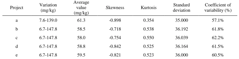
It can be seen from Table 1 that the average content of cultivated soil available phosphorus of Gaozhou is 59.5mg/kg, with variation of 6.7mg/kg-147.8mg/kg and up to more than 20 times among extremely poor values. In terms of skewness and kurtosis, the skewness of available phosphorus is -0.718 to -0.898, the data distribution and normal distribution of available phosphorus in the soil

sampling points deviate left relatively with kurtosis of 0.354 to 0.550. From coefficient of variability, with the change of sampling scale, the coefficient of variability of data of content of cultivated soil available phosphorus in Gaozhou is 57.1%-62.2%,

which belongs to medium variability strength[20];

[image:4.612.116.502.242.338.2]

seen from variation amplitude, the influence of sampling scale on the coefficient of variability of cultivated soil available phosphorus of Gaozhou is relatively small.

Table 1 Descriptive Statistics of Cultivated Soil Phosphorus Contents

Project Variation (mg/kg)

Average value (mg/kg)

Skewness Kurtosis Standard deviation

Coefficient of variability (%)

a 7.6-139.0 61.3 -0.898 0.354 35.000 57.1%

b 6.7-147.8 58.5 -0.718 0.538 36.192 61.8%

c 6.7-147.8 58.0 -0.754 0.550 36.039 62.2%

d 6.7-147.8 58.8 -0.842 0.525 36.164 61.5%

e 6.7-147.8 59.5 -0.821 0.523 36.000 60.5%

3.2 Analysis On Spatial Structure Of Soil Available Phosphorus

There exists a semi-variance structure in surface soil available phosphorus of Gaozhou in all the 5 projects, but there exists a certain difference of spatial variability in of available phosphorus in different projects (Table 2). In the 5 projects, only the training sample has 100% relatively matching of theoretical model with the index model and in other projects, the theoretical model of available phosphorus has a relatively matching with the

spherical model and the values of C0/(C1+C0) is

more than 75% in all projects and reaches the maximum in project d, up to 83.2%, indicating that available phosphorus has a weak structural space autocorrelation, the interference of structural factors to the spatial distribution is relatively small, there exists a spatial correlation in a

relatively large extent, the spatial gradual change is poor and the content of available phosphorus of surface cultivated soil is a little high and low in a small extent. This indicates that the fertilization of cultivated land, plants planted and management grade etc. have a very large influence on the spatial variability of soil nutrient. Seen from variation, project has the minimum main variation, 26947.9m, project has the maximum one, 67511.5m, the main variation direction of spatial variability is stabilized at about 315° and the proportion between primary and secondary variations is about 1.5, indicating that although the available phosphorus has a spatial autocorrelation in a relatively large extent, it is influenced greatly by direction and has different variability strengths in different directions.

Table 2 Semivariogram Parameter Of Soil Available Phosphorus Contents

Project Theoretical

model Anisotropism

Main variation

(a1, m)

Secondary variation

(a2, m)

Main direction

(°)

Nugget variance

(C0)

Structural variance

(C1)

C0/(C0+C1)

a

Exponential

model Y 26947.9 16298.2 306.3 27.252 6.839 79.9 %

b Spherical model Y 67511.5 37635.6 313.5 10.938 3.233 77.2%

c Spherical model Y 53769 32547.1 325.1 8.616 2.01 81.1%

d Spherical model Y 50595.4 30242.2 324.1 9.132 1.8497 83.2%

e Spherical model Y 64137.8 32905.6 325.0 9.5374 2.1611 81.5%

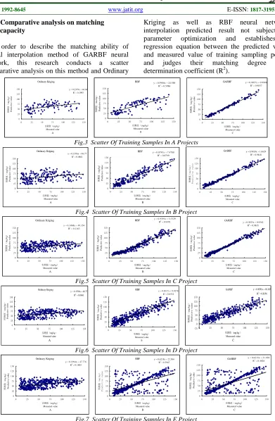
[image:4.612.92.527.580.682.2]

(5)

3.3.1 Comparative analysis on matching capacity

In order to describe the matching ability of spatial interpolation method of GARBF neural network, this research conducts a scatter comparative analysis on this method and Ordinary

Kriging as well as RBF neural network interpolation predicted result not subject to parameter optimization and establishes a regression equation between the predicted value and measured value of training sampling points and judges their matching degree with

determination coefficient (R2).

Ordinary Kriging

y = 0.2379x + 46.66 R2 = 0.1905

0 25 50 75 100 125 150

实测值（mg/kg） Measured value

A

预测值（

m g /k g ） P re d ic tiv e v a lu e

RBF y = 0.5986x + 24.588 R2 = 0.5986

0 25 50 75 100 125 150

B

预测值（

m a /k g ） P re d ic tiv e v a lu e

GARBF y = 0.9837x + 0.9988 R2 = 0.9837

0 25 50 75 100 125 150

C

预测值（

Fig.3 Scatter Of Training Samples In A Projects

Ordinary Kriging

y = 0.1596x + 48.77 R2 = 0.0861

0 25 50 75 100 125 150

A

预测值（

RBF _{y = 0.8743x + 7.4788} R2 = 0.8799 0 25 50 75 100 125 150

0 25 50 75 100 125 150

B

预测值（

m g/ kg ） P re d ic tiv e v a lu e

GARBF y = 0.9818x + 1.0629 R2_{= 0.9818}

0 25 50 75 100 125 150

C

预测值（m

g / k g ） Predictive value

Fig.4 Scatter Of Training Samples In B Project

Ordinary Kriging

y = 0.1468x + 49.354 R2 = 0.1163

0 25 50 75 100 125 150

A

预测值（

RBF y = 0.9391x + 3.5329

R2 = 0.9391

0 25 50 75 100 125 150

B

预测值（

GARBF

y = 0.9835x + 0.9562 R2 = 0.9835

0 25 50 75 100 125 150

C

预测值（

Fig.5 Scatter Of Training Samples In C Project

Ordinary Kriging

y = 0.1596x + 48.77 R2_{= 0.0861}

0 25 50 75 100 125 150

实测值（mg/kg） M easured value

A

预测值（

mg /k g ） P re di c ti ve va lue

RBF y = 0.8317x + 9.9278 R2 = 0.8332

0 25 50 75 100 125 150

B

预测值（

GARBF y = 0.8291x + 10.163 R2_{= 0.8356}

-25 0 25 50 75 100 125 150

0 25 50 75 100 125 150

C

预测值（

m g /k g ） P re d ict iv e v al u e

Fig.6 Scatter Of Training Samples In D Project

Ordinary Kriging

y = 0.1994x + 47.776 R2 = 0.1805

0 25 50 75 100 125 150

A

预测值（

m g/ kg ） P re d ic tiv e v a lu e

RBF y = 0.6218x + 22.506 R2 = 0.3967

0 25 50 75 100 125 150

B

预

测

值

（

mg/kg）

Predictive

value

GARBF y = 0.6315x + 21.928 R2_{= 0.4026}

0 25 50 75 100 125 150

C

预测值（

[image:5.612.116.507.68.666.2]

Fig.7 Scatter Of Training Samples In E Project

Figure 3-7 is the scattering distribution diagram of predicted value and measured value of training sampling points of cultivated soil available phosphorus of Gaozhou City obtained in 3 spatial

(6)

the matching capacities of the 3 methods all present different change trends. The predicted value of Kriging Method is the most approximate to the measured value in project a, determination

coefficient R2 is 0.1905, the determination

coefficients of (R2) regression equitation of

predicted values and measured values of neighbor point-based RBF neural network and GARBF neural network reach the maximum when the numbers of samples are respectively 200 and 100

and determination coefficients ((R2)) are

respectively 0.8799 and 0.9837.

3.3.2 Comparative analysis on interpolation error

Figure 4.8 shows the approximate error comparison of training samples of 3 spatial interpolation methods in the 5 projects of cultivated soil available phosphorous. Approximate error reflects the capacity of matching of training samples of interpolation methods with the known sampling points, which can compare with the matching result of regression equation in the scatter diagram of predicted value and measured value. It can be known from Figure 89 that in the 5 projects of rapidly available potassium, the mean absolute error (MAE) and root-mean-square error (RMSE)of GARBE neural network matching are less than those of the other 3 interpolation methods in Projects a, b and c, while in Projects d and e, there is basically no gap of MAE and RMSE between neighbor point-based RBF and GARBF neural network matching, both the MAE and RMSE of Ordinary Kriging matching are relatively large in the 5 projects. In the first three projects, the matching capacity of GARBF neural network is obviously better than that of the other two methods. With the increasing of training samples, the MAE and RMSE of matching of the 3 interpolation method are all fluctuated in some extent, in which neighbor point-based RBF neural network has the largest fluctuation, followed by GARBF neural network, while Ordinary Kriging has the smallest fluctuation. The MAE and RMSE of GARBF neural network matching are the minimum when the number of training samples is 100, with the increasing of samples, the MAE and RMSE of matching present an increasing trend; the MAE and RMSE of neighbor point-based neural network matching are the minimum when the number of training samples is 300, with the increasing of training samples, both MAE and RMSE increase and when the number of training samples reaches 500, the MAEs of the three methods are basically in the same grade, while the RMSEs of neighbor

point-based RBF and GARBF neural network matching are basically equal, but are less than the values of Ordinary Kriging.

Input the detection sampling points into neighbor point-based RBF model and genetic algorithm modification neighbor point RBF model for calculation, meanwhile export the predicted values of detection sampling points obtained through Ordinary Kriging interpolation method in ArcGIS and then verify the spatial interpolation capacity of the three methods.

It can be seen from Figure 9 that in the 5 projects of available phosphorous, the MAE and RMSE of detection samples of GARBF neural network are always less than those in the other three methods, indicating the interpolation accuracy and reliability of GARBF neural network are better than the other two methods. Expect that the RMSE of neighbor point-based neural network is approximate to that in Ordinary Kriging method, it is more than that in Ordinary Kriging in the rest 4 projects and the fluctuation of MAE is also relatively large, indicating that the stability of spatial interpolation of neighbor point-based RBF neutral network is relatively poor. With the increasing of training samples, the MAE and RMSE of detection samples of the three interpolation methods are all fluctuated in some extent. In the three methods, the MAE and RMSE of detection samples reach the minimum when the number of training samples is 400, and then present an increasing trend, but keep the state of GARBF neutral network> Ordinary Kriging >neighbor point-based RBF neural network.

3.4 Spatial Pattern Of Cultivated Soil Available Phosphorous Of Gaozhou City And Analysis On The Cause Of Formation

As the most available part to crops in cultivated soil available phosphorus deposit, available phosphorus can be directly absorbed and utilized by crops, so it is an important factors to evaluate the

cultivated soil phosphorous supply capacity[23].

(7)

threat to the ecological environment[24-27]. The content range of cultivated soil available phosphorous of Ganzhou is 1.352-153.582mg/kg, according to the grade statistics of cultivated soil available phosphorous (Figure 10, Table 3), the area of cultivated land with soil available phosphorous content Grade I is

32687.319hm2,, accounting for 55.871% of the total

cultivated land area and the distribution of cultivated land of this grade can be found in each town of Gaozhou and in some towns, the content of available phosphorous of all cultivated soils is above Grade 1, with serious surplus. The area of cultivated land with soil available phosphorous

content Grade II is 17714.247hm2, accounting for

30.278% of the total land, which is mainly distributed in towns such as Zhenjiang, Shigu, Shatian, Hetang, Hehua and Tantou. The area of cultivated land with soil available phosphorous content Grade III is 6699.801hm2, accounting for 11.452% of the total cultivated land, the cultivated land of this grade is distributed messily, mainly distributed in each town in the east. The areas of cultivated land with soil available phosphorous contents Grades IV, V and VI are respectively

1199.219 hm2, 94.913 hm2 and 109.501 hm2,

accounting for not less than 3% of total cultivated land area of Gaozhou. Due to high agricultural production intensification in Gaozhou, together with the fact that Gaozhou is located in red soil,

latosolic red soil and laterite areas with large

cultivated area of acid soils. These soils contain numerous soil components such as amorphous alumina, making cultivated soil rapid available

phosphorous lack very much[28], and this increases

[image:7.612.322.536.391.565.2]

the fertilization strength. It is found in the investigation that generally farmers will apply phosphoric fertilizer greatly and then apply compound fertilizer and organic fertilizers such as animal dung again according as needed by the crops, but the utilization of phosphoric fertilizer is relatively low, making phosphorous element accumulate in soil greatly and extremely high surplus occurs to cultivated soil available phosphorous.

Table 3 The Grades Statistics Of Cultivated Soil Available Phosphorus Contents In Gaozhou City

Available phosphorous grade

Content (mg/kg)

Area (hm2) Proportion (%)

Grade I >40 32687.319 55.87

Grade II 20-40 17714.247 30.28

Grade III 10-20 6699.801 11.45

Grade IV 5-10 1199.219 2.05

Grade V 3-5 94.913 0.16

Grade VI 0-3 109.501 0.19

4. CONCLUSION AND DISCUSSION

[image:7.612.91.301.634.726.2]

There exists a semi-variance structure in surface cultivated soil available phosphorous of Gaozhou. In the 5 projects, only the optimal matching model of semi-variance function of soil available phosphorous in project a is index model and the models in other projects are all spherical models; in the 5 projects, the semi-variance function curve of available phosphorus has a better matching with the theoretical model curve, which fits the index or spherical model very much; meanwhile, in each project, the curve change of available phosphorous is also relatively strong, indicating that it is influenced greatly by the small-scale influential factors, there exists spatial correlation in a larger extent with poor spatial gradual change and the content of soil available phosphorus is a little high and low in a small extent, indicating that the fertilization of land, plants planted and management level etc. have a very great influence on then spatial variability of surface cultivated soil available phosphorous.

Fig.10 The Distribution Of Cultivated Soil Available Phosphorus Contents In Gaozhou City

In terms of matching capacity, GARBF neural network spatial interpolation is better than other two methods. With the increasing of training samples, the matching capacities of the three methods present different change trends, but the overall trend is first increasing and then reducing. In terms of MAE and RMSE of predicted value and measured value, the MAE and RMSE of GARBF are obviously less than those of the other two methods, and under the condition that there are few

(8)

interpolation, the interpolation capacity of GARBF neural network presents an obvious advantage, indicating that GARBF neural network has the strongest interpolation capacity in the three methods and reflecting the strong non-linear mapping capacity of GARBF neural network. With the increasing of training samples, the MAE and RMSE obtained from the three interpolation methods are all fluctuated in some extent and in the 5 projects, the neighbor point-based RBF neural network has the largest fluctuation, followed by GARBF neural network, while Ordinary Kriging has no fluctuation basically.

This researches uses genetic algorithm to optimize such parameters as the number of implicit node, expansion speed and root-mean-square error of RBF neural network and adopts binary coding as the coding system of gene and takes roulette model as the realization model of natural selection of genetic algorithm. The research shows that the spatial interpolation capacity of RBF neural network through optimization of genetic algorithm is better than the geostatistics and neighbor point-based RBF neural network method and it is more obvious when there are fewer interpolation sampling points. As there exists a very complex non-linear relation between the cultivated soil characteristics and various influential factors, if relevant factors such as soil parent material, planting system, fertilization methods, elevation and other nutrient factors influencing the sample property can be blended into the network when the neural network interpolation is used, it can not only improve the network stability and interpolation accuracy but can also realize the synchronous difference of multi-property of soil. Meanwhile, the training samples of each project are increased by 100 gradually, with relatively large spacing, if the spacing can be reduced, it will be easier to find the change trend of number of training samples participating in the interpolation and interpolation accuracy, so as to accurately find out the reasonable sampling points of spatial interpolation of regional soil property and further save the research cost.

REFRENCES:

[1]Holford R. I. C. Soil phosphorus: its measurement, and its uptake by plants [J]. Australian Journal of Soil Research, 1997,35(2):227-240.

[2]Hooda P S, Truesdale V W, Edwards A C, et al. Manuring and fertilization effects on

phosphorus accumulation in soils and potential environmental implications[J]. Advances in Environmental Research,2001,5(1):13-21. [3]Hechrath G, Brookes C P, Poulton R P, et al.

Phosphorus leaching from soils containing different phosphorus concentrations in the Broadbalk experiment [J]. Journal Environmental Qualty,1995(24): 904-910.

[4]Van Der Molen D T, Breeuwsma A, Boers M P C. Agricultural nutrient losses to surface water in the Netherlands: Impact, strategies, and perspectives[J]. Journal of Environmetal Quality,1998,27(1):4-11.

[5]Yuan Donghai, Wang Zhaoqian, Chen Xin, et al. Characteristics of phosphorus losses from slop field in red soil area under different cultivated ways[J]. Chinese Journal of Applied Ecology, 2003,14(10):1661-1664.

[6]Li Xiaoyan, Zhang Shuwen, Wang Zongming, et al. Spatial variability and pattern analysis of soil properties in Dehui City of Jilin Province[J]. Acta Geographica Sinica,2004,59(6):989-997. [7]Shen Zhangquan, Zhou Bin, Kong Fansheng, et

al. Study on spatial variety of soil properties by

means of generalized regression neural

network[J].Acta Pedologica Sinica, 2004, 41(3): 471-475.

[8]Dong Min, Wang Changquan, Li Bing, et al. Study on soil available zinc with GA-RBF-Neural-Network-Based spatial interpolation method[J]. Acta Pedologica Sinca,2010,47(1):42-50.

[9]Numata I, Soares J V, Roberts D A, et al. Relationships among soil fertility dynamics and remotely sensed measures across pasture chronosequences in Rondônia, Brazil[J]. Remote Sensing of Environment,2003,87(4): 446-455.

[10]Li Xinyu, Yu Wantai, Li Xiuzhen. Comparison and application of remote sensing and geistatistics methods to spatial distribution of surface soil organic carban[J]. Transactiond of the CSAE,2009,25(3):148-152

[11]Lian Gang, Guo Xudong, Fu Bojie, et al. Prediction of spatial distribution of soil properties based on environmental correlation and geostatistics[J]. Transactions of the CSAE,2009,25(7):237-242.

(9)

Conference on Systems, Man and Cybernetics,2000,4:2673-2678.

[13]Shen Zhangquan, Shi Jiebin, Wang Ke, et al. Spatial variety of soil properties by BP neural network ensemble[J]. Transactions of the CSAE,2000,4:2673-2678.

[14]Wang Xudong, Shao Huihe. The theory of RBF neural network and its application in control[J]. Information and Control,1997,26(4):272-284. [15]Pan Yuchun, Liu Qiaoqin, Yan Bojie, et al.

Effects of sampling scale on soil nutrition spatial variability analysis[J]. Chinese Journal of Soil Science,2010,41(2):257-262.

[16]Broomhead D S. Multivariable functional interpolation and adaptive networks[J]. IEEE International Conference on Complex Systems,1988,2:321-355.

[17]Hartman J E, Keeler D J, Kowalski J. Layered neural networks with Gaussian hidden units as universal approximations[J]. Neural Computation,1990,2(6):210-215.

[18]Qu N, Wang L, Zhu M, et al. Radial basis function networks combined with genetic algorithm applied to nondestructive determination of compound erythromycin ethylsuccinate powder[J]. Chemometrics and Intelligent Laboratory Systems,2008,90(2):145-152.

[19]Wang Chengzhang, Yin Bocai, Sun Yanfeng, et al. An improved 3D face-modeling method based on morphable model[J]. Acta Automatica Sinica,2007,33(3):232-239.

[20]Lei Zhidong, Yang Shixiu, Xu Zhirong, et al. Preliminary investigation of the spatial variability soil properties[J]. Shui Li Xue Bao,1985(9):10-21.

[21]Cambardella A C, Moorman B T, Novak M J. Field-scale variability of soil properties in central lowa soils[J]. Soil Science Society of America Journal,1994,58:1240-1248.

[22]Chien Y, Lee D, Guo H, et al. Geostatistical analysis of soil properties of mid-west Taiwan soils.[J]. Soil Science,1997,162(4):291-298. [23]Liao Jingjing, Huang Biao, Sun Weixia, et al.

Spatio-temporal variation of soil available phosphorus an its influencing factors—a case study of Rugao County, Jiangsu Province[J], Acta Pedologica Sinica,2007,44(4):620-628. [24]Liu Jianling, Liao Wenhua, Zhang Zuoxin, et al.

The response of vegetable yield to phosphate fertilizer and organic manure and environmental risk assessment of phosphorus accumulated on

soil[J]. Scientia Agricultura Sinca,2007,40(5):959-965.

[25]Sharpley N A, Mcdowell W R, Kleinman A P J. Amounts, Forms and Solubility of Phosphorus in Soils Receiving Manure[J]. Soil Science Society of America Journal,2004(68):2048-2057.

[26]Brus D J, Spjens L E E M, de Gruijter J J. A sampling scheme for estimating the mean extractable phosphorus concentration of fields for environmental regulation[J]. Geoderma.1999,89(1-2): 129-148.

[27]Wang Shuying, Hu Kelin, Liu Ping, et al. Spatial variability of soil phosphorus and environmental risk analysis of soil phosphorus in Pinggu County of Beijing[J]. Scientia Agricultura Sinca, 2009,42(4):1290-1298. [28]Zhang Xinming, Li Huaxing, Liu Jinyuan.

(10)