Hardening against adversarial examples with the smooth gradient method

(1)

BIROn - Birkbeck Institutional Research Online

Mosca, Alan and Magoulas, George D. (2018) Hardening against adversarial

examples with the smooth gradient method. Soft Computing 22 (10), pp.

3203-3213. ISSN 1432-7643.

Downloaded from:

Usage Guidelines:

Please refer to usage guidelines at

or alternatively

(2)

(will be inserted by the editor)

Hardening against adversarial examples with the Smooth

Gradient Method

Alan Mosca _· George D. Magoulas

Received: date / Accepted: date

Abstract Commonly used methods in Deep Learning do not utilise transfor-mations of the residual gradient available at the inputs to update the represen-tation in the dataset. It has been shown that this residual gradient, which can be interpreted as the first order gradient of the input sensitivity at a particular point, may be used to improve generalisation in feed-forward neural networks, including fully connected and convolutional layers. We explore how these in-put gradients are related to inin-put perturbations used to generate adversarial examples, and how the networks that are trained with this technique are more robust to attacks generated with the Fast Gradient Sign method.

1 Introduction

Most supervised Deep Learning models are trained with backpropagation [22, 6], and different variants of Gradient Descent. The main principle upon which this methodology is based is the application of a so-calledweights update rule, which uses an error gradient with respect to the internal parameters of the model

∆Wt=∇E(Wt) (1)

We gratefully acknowledge the support of NVIDIA Corporation with the donation of the GTX Titan X GPUs used for this research.

Alan Mosca

Department of Computer Science and Information Systems, Birkbeck, University of London, Malet Street, London WC1E 7HX, E-mail: [email protected]

George D. Magoulas

(3)

at training epocht, whereWtare the parameters of the hypothesish(Wt, X)

being optimised, where X = {x1,x2, . . . ,xm} is the input matrix. Such an

update rule∆Wt is used to produce an incremental parameter change:

Wt+1=Wt−λ∇Et(Wt) (2)

where λ is usually called the learning rate. The function Et generates the

values of the error function at timet, sometimes also referred to as thecost function.

For simplicity of notation, we indicate nodes with a single index, rather than identifying them by layer and position in the layer. In practice, when considering Artificial Neural Networks trained with back-propagation, each parameter wki→lj,t, which represents the weight connecting the i-th node of

the k-th layer to the j-th node of the l = (k+ 1)-th layer, ∀l ∈ 1, ...N is updated by considering the corresponding element of the Jacobian i.e the partial derivative

∂Et

∂wki→lj,t

(3)

of the error functionEtwith respect to each weight. This information is used

in the calculation ofwki→lj,t+1.

When back-propagated, the calculation of the partial derivative of Equa-tion (3) is based on applicaEqua-tion of the chain rule, as shown in EquaEqua-tion (4) below, and typically stops at the first/input layerk= 0. N is the number of layers in the network.

∂Et

∂w0i→1j,t

= ∂w1i→2j,t

∂w0i→1j,t

. . . ∂w(N−1)i→N j,t ∂w(N−2)i→(N−2)j,t

∂Et

∂w(N−1)i→N j,t

(4)

The term ∂w1i→2j,t

∂w0i→1j,t of the equation is some times calledinput sensitivity. If we abbreviate this term asSt, then we can reformulate Equation (4) in terms

of the input sensitivity, as shown in Equation (5):

∂Et

∂w0i→1j,t

=St

∂w2i→3j,t

∂w1i→2j,t

. . . ∂w(N−1)i→N j,t ∂w(N−2)i→(N−1)j,t

∂Et

∂w(N−1)i→N j,t

=St

∂Et

∂w1i→2j,t

(5)

1.1 Deep Neural Networks

Deep Neural Networks (DNN) follow basic principles of traditional Artificial Neural Networks but include a large number of layers. An example of such a methodology is shown in Ref [2].

(4)

functionϕ(x)1_{, then the output}_o

lj,t of a nodej in a hidden layerl at timet

of a DNN is

olj,t=ϕ(netlj,t) =ϕ n

X

i=1

wki→lj,toi

!

(6)

and the derivative of the error with respect to the weights of a node in the output layer can be rewritten as

∂Et

∂wki→lj,t

= ∂Et

∂olj,t

∂netlj,t

∂wki→lj,t

. (7)

For allnnodes in the previous layeri=l−1, the last term becomes

∂netlj,t

∂wki→lj,t

= ∂

∂wki→lj,t n

X

z=1

wkz→lj,tokz,t

!

=oki,t. (8)

The second term becomes

∂olj,t

∂netlj,t

= ∂

∂netlj,t

ϕ(netlj,t) (9)

and for each nodepin a layerq, the first term becomes

∂Et

∂olj,t

= X

q=1→l−1 X

p∈q

∂Et

∂netqp,t

∂olj,t

= X

q=1→l−1 X

p∈q

∂Et

∂oqp,t

∂netqp,t

wmp→lj,t

,

(10)

1.2 Convolutional Neural Networks

Convolutional Neural Networks [12] are normally composed of two parts: con-volution and pooling. Concon-volution creates a sliding window over the input space which is convolved to learn a shared set of weights that produces a smaller output. Pooling reduces the number of features by selecting only the maximum out of a pre-definedpool of the outputs of the convolutional step. For convenience we consider convolution in two dimensions, however the pro-cedure can be extended to an arbitrary number of dimensions.

If we consider anN×M rectangular output from layer nodeiin layerkto nodej in layerl, to which an×mrectangular kernelWki→lj,tis applied, the

forward pass of the convolution operation to produce an output value olj,t,

after applying an activation functionϕ(·), yields:

olj,t=ϕ n−1 X

a=0

m−1 X

b=0

wabok(j+{a,b}) !

, (11)

1

(5)

where wki→lj,ab,t is the weight contained in the kernelW at coordinatesa, b,

and j = {j0, j1} are the coordinates of the output value. This makes the

gradient more complex, but still computable:

∂Et

∂wki→lj,ab,t

=

n−1 X

a=0

m−1 X

b=0

∂Et

∂olj,t

∂wki→lj,ab,t

=

n−1 X

a=0

m−1 X

b=0

∂Et

∂olj,t

ϕ′ ok(j+{a,b},t

ϕ ok(j+{a,b},t

(12)

this can be propagated backwards, obtaining:

∂Et

∂okj,t

=

n−1 X

a=0

m−1 X

b=0

∂Et

∂ol(j−{a,b}),t

∂okj,t

=

n−1 X

a=0

m−1 X

b=0

∂Et

∂ol(j−{a,b}),t

wki→lj,ab,t

(13)

The rest of the paper is structured as follows. Section 2 explores the theory behind the technique and introduces new considerations in merit. Section 3 ex-plores the relationship between learning input representations and adversarial examples. Section 4 extends the theory to random perturbations of the input (such as random noise). Section 5 shows experimental results on benchmark datasets in computer vision. Section 6 shows experimentally how the networks generated develop a higher robustness to adversarial examples, and Section 7 draws final conclusions about the technique and the associated experimental results.

2 Backpropagating the error to the input

By the same principle, the chain rule can be applied once more, obtaining a new partial derivative of the error with respect to the specific representation of each component of the input matrixXat epocht, as shown in Equation (14). We call this theresidual error gradient at the inputs.

∂Et

∂xi,t

= ∂Et

∂w0i→1j,t

∂xi,t

. (14)

wherew0i→1j,tis the weight that connects inputito nodej in the first layer.

(6)

This approach has been further developed in Ref [17], where the principle of applying one further step of backpropagation to obtain an update of the inputs in convolutional and fully-connected deep neural networks has been introduced. The authors also provide a proof of computability of the residual error of Equation (14). An important caveat is that, because ∂Et

∂xi,t is determined analytically, the proof does not hold when random perturbations of the input are present, such as random noise injection or elastic transformations [23]. We will however show that, when the random perturbations are designed to have a mean converging towards zero, this approach can still be applied, and as our experiments confirm, it is able to still provide comparable generalisation capability.

The residual error of Equation (14) can be utilised to update the value of the inputs at each training epoch to increase the speed of convergence, with the goal of maximising the internal gradients of the network at the following epoch t+ 1. Furthermore, because we are operating on the very first inputs into the network, we do not need to distinguish between different types of networks.

Therefore an iterative scheme to adapt the input representations at each time steptcan be expressed as

Xt+1=Xt+ ¯λ∇Et(Xt), (15)

where ¯λis a choseninput update learning rate. While previous work [17] recom-mended that 0≤λ¯≤1 and a value of ¯λ= 1 worked well in our experiments, after further experimentation we found that values in the range−1 ≤λ¯ ≤1 also work well and that the best available value of ¯λcan be searched by hy-perparameter optimisation.

3 Relationship to adversarial examples

Adversarial Examples [25] are a particular type of learned input perturba-tion that, although being imperceptible to the human eye, and therefore very small in magnitude when compared with the undisturbed input values, are able to modify the output of a neural network significantly. In some cases these examples have been likened to the neural network’s equivalent of an op-tical illusion. In Ref [4] the authors attempt to explain this phenomenon in terms of the linear nature of the neural networks, and provide an example of how such examples can be generated. In Ref [19] the authors illustrate how such examples could become dangerous, especially as deep learning and neural networks become more prominent in the modern technological landscape.

(7)

The generation of such adversarial examples relies on the attacker having access to the gradients of the model. However, several approaches aimed at hiding this gradient, sometimes called “gradient masking”, have been shown to not be effective at reducing the sensitivity to these examples [19].

Given that the approach towards generating and protecting from adversar-ial examples is very similar to that of adapting the input representations, as explained in Ref [17], we analyse the relationship between the two approaches. In both cases, there is an original traning examplexm, taken from a

train-ing set X, which is then combined with a perturbation υm, which is static

with respect to the final network for generating an adversarial example x˜m,

and pertains to the current training epoch in the case of input updates xi,t,

taking the form ofυi,t. Equation (16) shows the approach for adversarial

ex-amples, whilst Equation (17) shows the related expression for the training input updates.

˜

xm=xm+υm (16)

xi,t+1=xi,t+υi,t (17)

Because of the similarity between Equation (16) and Equation (17), a more general notation that applies to both cases can be used to derive the expression in Equation (18), for the entire training set, with the special case that for updated inputs at each epoch,Xt+1= ˜Xt.

˜

Xt=Xt+Υt (18)

In both cases, we know thatΥ is derived from the gradients of the model, defined as sensitivity of the model with respect to the input changes, as shown in Equation 19, whereF(·) is some arbitrarily chosen function.

Υ =F(∇E(Xt)) (19)

3.1 Current approaches

In the so-called “Fast Gradient Sign method” [4] for generating the adversarial examples, the sign of the partial derivatives of the cost with respect to the input is applied as an input perturbation, as shown in Equation (20). It is to be noted that the notation used by the authors is different from that used in this paper, and a translated version to the notation used in this paper is provided instead.

˜

xi,t=xi,t+ ¯λsgn

∂Et

∂xi,t

(20)

(8)

reversal layer” to ensure that feature distributions over the source and target domains are made similar. This type of approach, whilst not explicitly targeted at adversarial examples, illustrates that other solutions may exist that are not based on modified input values.

3.2 A smooth approach

By following the method prescribed in Ref [17], we are adding the partial derivative with respect to the input to the input itself at each epoch, multiplied by a learning rate ¯λ, Equation (21), therefore forcing the network to reduce its sensitivity to these variations, by forcing larger updates during the following round.

xi,t+1=xi,t+ ¯λ

∂Et

∂xi,t

(21)

If we discard the application of the sgn(·) function, the relation between the two operations is self-evident. Training the network on inputs that are continuously updated to reduce the sensitivity to the gradient of the error with respect to the input can therefore be considered equivalent to the continuous online creation of new adversarial examples at each training iterarion, against which the network is hardened. This approach, which we call the Smooth Gradient Method (SGM) leads to more robust networks and in some cases it is also able to increase traning speed and accuracy.

By not applying the sgn(·), the input perturbations are no longer limited to the domain{−λ,¯ λ¯}, but are instead able to extend to the entire domain of

R.

4 Extension to random perturbations

For a learning setting with random noise perturbations, we must consider the asymptotic effect of the additional factorǫtand how it will impact the

consid-erations made for the improvements in training. It has been shown that under certain conditions the addition of particular types of training noise to the train-ing data is very useful to improve the traintrain-ing performace [23]. Previous work has been done to prove the convergence on perturbations in back-propagation, and the goal of this section is to illustrate how the concept applies to the per-turbation ǫt. We assume that ǫt is a random, stationary ergodic process (in

most cases of perturbations this actually the case). This will make the sequence ofX0...Xt a stationary process.

If one extends Equation (18) to include a perturbation from random affec-tations of the training setǫt, caused by a noisy learning process at epoch t,

one can obtain the formulation of Equation (22).

(9)

A brief explanation of why both the FGSM method and SGM work in a noisy setting is provided.

We begin by considering the simpler case for Xt+1 =Xt+ǫt. At epoch

t, we expect that the gradient of the error with respect to the current input will be, in expectation, similar to the error with respect to the original input X0=X.

For an input xi,t ∈Xt, we assume our distribution of each perturbation

ǫi,t∈ǫtto also have zero-mean and be symmetric such that

E[ǫt] = 0 (23)

and the variance to be such that its sum overtconverges to a finite number.

t

X

k=0

Var (ǫt) =s (24)

Most random noise is of this kind, as it is usually generated from samples from a gaussian distribution. We also know that

Xt+1=Xt+ǫt (25)

If we then unroll the recursive relationship in Equation (25), we obtain

Xt+1=X0+ǫ0+ǫ1+· · ·+ǫt−1+ǫt (26)

or, more simply

Xt+1=X0+

t

X

k=0

ǫk (27)

We can then rewrite our problem statement as

E " _t

X

k=0

∂Ek

∂Xt

# =E   t X k=0 ∂Ek

∂X0+Pt_k=0ǫk



=E   t X k=0 ∂Ek

∂X0+E h

Pt

k=0ǫk

i 



(28) By the definition of its distribution, we know that

E " _t X k=0 ǫk # = t X k=0

E[ǫk] = 0 (29)

and that this is admissible because we restricted the sequence of allǫtto have

a cumulative converging variance (Equation 24, therefore allowing that

E " _t

X

k=0

∂Ek

∂Xt

# ≈E " _t X k=0 ∂Ek

∂X0 #

(30)

(10)

E[∇Et(Xt)]≈E

"

∇Et X0+

t X k=0 Υk !# (31)

and simplified to

E[Xt]≈E

"

X0+

t X k=0 Υk # (32)

From a similar unrolling procedure to Equation (26), we can derive that

Xt=X0+

t

X

k=0

Υk+ t

X

k=0

ǫk (33)

and by Equation (29)

E "

X0+

t

X

k=0

Υk+ t X k=0 ǫk # =E "

X0+

t X k=0 Υk # (34)

which in turn allows for

E[Xt] =E

"

X0+

t X k=0 Υk # (35)

Therefore the original statement in Equation (32) can be considered valid.

5 Experimental analysis

The input update technique has been tested on some common benchmark computer vision datasets, frequently used to compare the performance of Deep Learning algorithms. Using computer vision tasks allows us also to visualise the gradients propagated back to the input, the updated inputs and the adversarial examples in a human–friendly manner. Our experimental methodology consists of running the same Convolutional Neural Network five times and reporting the median results. This is the same methodology as reported in [24]. We chose this methodology because it is in line with other results on the same datasets, and it allows us to produce effective results even in the case where the training is a very slow process2_{. We first generate our control experiment}

without augmenting the input, and we then repeat the same experiments with the updates enabled. For consistency, the random initializations are fixed to be in lock-step: theNth run of each of the both variants of the architecture would receive the same initialisation.

For all network types we used the WAME weight update rule [18], which has been shown to have good properties of fast convergence on Convolutional Neural Networks.

2

(11)

2500 fully-connected nodes 50% dropout 2000 fully-connected nodes

50% dropout 1500 fully-connected nodes

50% dropout 10 way softmax

Table 1: The fully-connected network structure used for the MNIST dataset.

For the input update methodology, after experimental tuning of hyperpa-rameters, an input learning rate of ¯λ= 0.2 was used to maximise the robust-ness to adversarial examples.

5.1 Datasets

The datasets used for comparing our technique are common computer vision datasets, frequently used to compare performance of supervised Deep Learning methods. They are as follows.

5.1.1 MNIST

MNIST [13] is a common computer vision dataset that associates pre-processed images of hand-written numerical digits with a class label representing that digit. The input features are the raw pixel values for the 28×28 images, in grayscale, and the outputs are the numerical value between 0 and 9. There are 50000 training images, 10000 validation images and 10000 test images.

For this dataset, we tested both a Deep Neural Network built only with fully-connected layers, and a Convolutional Neural Network.

Fully-connected Deep Neural Networks: For the Fully-connected version of the MNIST network, we used the network structure shown in Table 1.

All layers used batch normalization [9].

Figure 1 shows that the mean test misclassification at each epoch closely tracks that of the control experiment, and then continues to be reduced after the control experiment has stopped improving.

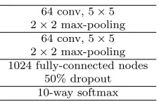
Convolutional Neural Networks: For the Convolutional version of the MNIST network we used the structure illustrated in Table 2.

(12)

1.4 1.6 1.8 2 2.2 2.4 2.6 2.8 3 3.2

0 2 4 6 8 10 12 14 16

Test Error (%)

Training Epoch

[image:12.595.73.406.73.302.2]

w/o input update (1 std) w/ input update (1 std)

Fig. 1: Test misclassification rate - DNN on MNIST, without dataset augmentation

64 conv, 5×₅

2×2 max-pooling

64 conv, 5×₅

2×2 max-pooling

[image:12.595.185.298.345.418.2]

1024 fully-connected nodes 50% dropout 10-way softmax

Table 2: The convolutional network structure used for the MNIST dataset.

Figure 2 shows that the mean test misclassification at each epoch during the initial phase of the learning closely tracks that of the control experiment, and is in most cases marginally better.

5.1.2 CIFAR-10

(13)

0.4 0.5 0.6 0.7 0.8 0.9 1

0 2 4 6 8 10

Test Error (%)

Training Epoch

[image:13.595.73.401.73.300.2]

w/o input update w/ input update

Fig. 2: Test misclassification rate - CNN on MNIST, without dataset augmentation

2×96 conv, 3×3

96 conv, 3×3, 2×2 strides

96 conv, 3×_{3, 2}×_{2 strides}

2×2 max-pooling

2×192 conv, 3×3

2×2 max-pooling *

192 conv, 3×3

192 conv, 1×1

10 conv, 1×1

global average pooling 10-way softmax

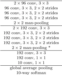
Table 3: The network structure used for the CIFAR-10 dataset.

The CNN we used for CIFAR-10 is a variant of the model used in Ref [15], which is a relatively small network that reaches a very good accuracy in a short training time. Its structure is illustrated in Table 3.

5.1.3 CIFAR-100

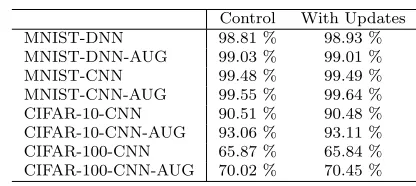
[image:13.595.180.300.345.489.2]

(14)

Control With Updates MNIST-DNN 98._{81 %} ₉₈._{93 %}

MNIST-DNN-AUG 99._{03 %} ₉₉._{01 %}

MNIST-CNN 99._{48 %} ₉₉._{49 %}

MNIST-CNN-AUG 99._{55 %} ₉₉._{64 %}

CIFAR-10-CNN 90._{51 %} ₉₀._{48 %}

CIFAR-10-CNN-AUG 93._{06 %} ₉₃._{11 %}

CIFAR-100-CNN 65._{87 %} ₆₅._{84 %}

[image:14.595.133.341.85.178.2]

CIFAR-100-CNN-AUG 70._{02 %} ₇₀._{45 %}

Table 4: Test accuracy on the benchmark datasets for the methods compared. DNN indicates a fully-connected Deep Neural Network, CNN indicates a Convolutional Neural Network, whilst AUG indicates that dataset augmentation was used.

image format is the same as CIFAR10. Class labels are provided for the 100 classes as well as the 20 super-classes. A super-class is a category that includes 5 of the fine-grained class labels (e.g. “insects” containsbee, beetle, butterfly, caterpillar, cockroach). Of the 60000 samples, there is a training set of 40000 instances, a validation set of 10000 and a test set of another 10000. All sets have perfect class balance.

The model we used was the same as that used for the CIFAR-10 dataset, illustrated in Table 3.

5.2 Data augmentation

The augmentation of available data with additional derived examples, such as from linear transformation (flip, rotate, zoom, random cropping) or more complex ones, is a common practice with all the datasets used in this paper. In the case of MNIST, the application of dataset augmentation practices is indeed very common. A specialised methodology, called elastic distortions [23], has been frequently used in conjunction with this dataset, to generate a virtually-infinite training dataset in an “online” fashion. At each epoch a new distorted version of the training set is created, by simulating hand jitters and other linear imperfections. In our results we include both augmented and non-augmented versions of the dataset, for both types of networks.

For CIFAR-10 and CIFAR-100, we utilised ZCA Whitening as a preprocess-ing method, and then used a light augmentation schedule of random rotations, zoom, and random horizontal flips. We did not use any random cropping.

5.3 Results

(15)

values have been actually improved slightly. In addition, a Wilcoxon test re-jects the hypothesis that the two experiments are significantly different with respect to this accuracy measurement. It has been shown in the literature [17] that using ¯λ = 1 would make such an improvement significant, and as such our preference for optimising this hyperparameter has been given to learning robustness to adversarial examples.

6 Testing robustness to adversarial examples

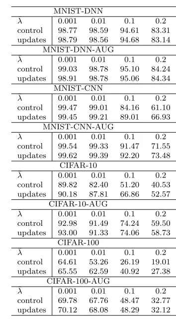
We constructed an adversarial test set, following the procedure explained in [4]: we added perturbations to the original test set, based on the Fast Gradient Sign method, and tested accuracy of predictions for each model based on the dataset. We then compared how each of the trained models fared on this new test set. We used different values of ¯λ = 0.001,0.01,0.1,0.2 for comparison with small and large perturbations.

Results are compiled in Table 5. A Wilcoxon paired test shows that the improvements on adversarial examples are statistically significant at the 0.005 confidence level, giving strong reason to suggest that using the input update method is able to improve robustness to adversarial examples generated with the Fast Gradient Sign method.

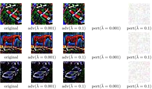
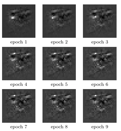
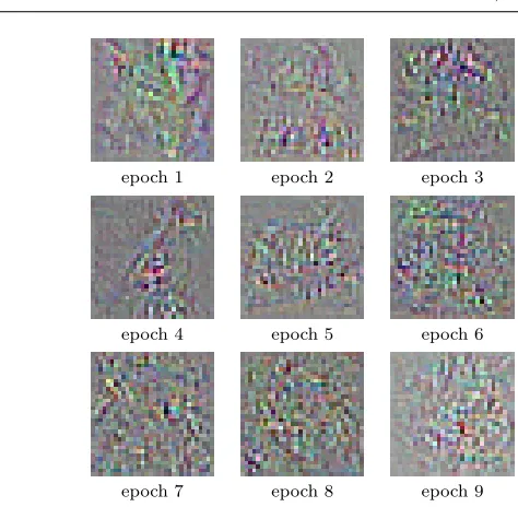
The images in Figures 3 and 4, show images that have been misclassified by the original classifier, but have been correctly classified by the classifier hardened using our method. The adversarial images are still clearly visible as their original class by the human eye, whilst the classifier is making significant mistakes – for example the airplane in Figure 4 is being classified asautomobile at both levels of ¯λbeing shown. An image of the perturbations alone is also included, for reference. Even though the figures have been inverted to make the distortions more evident, in many cases they are still mostly imperceptible. Figures 5 and 6 show examples of backpropagated input distortions during the first nine epochs, for MNIST and CIFAR-10 respectively. It is of note that the updates to the input appear to be small in magnitude, but nonetheless their effect is noticeable3_.

7 Conclusions

We have shown how adapting the input representations based on the residual gradient of the error with respect to the inputs at time t, is not only an effective technique for increasing the speed of convergence and overall learning capability of an Artificial Neural Network, as was previously shown by Ref [17], but that the application of this process with a smaller input learning rate ¯λ

3

50% grey indicates no update, whilst white indicates an update value of +1 and black indicates an update value of−1. For CIFAR-10, the three separate colour channels have

(16)

MNIST-DNN ¯

λ ₀.₀₀₁ ₀.₀₁ ₀.₁ ₀.₂

control 98.₇₇ ₉₈.₅₉ ₉₄.₆₁ ₈₃.₃₁

updates 98.₇₉ ₉₈.₅₆ ₉₄.₆₈ ₈₃.₁₄

MNIST-DNN-AUG ¯

λ ₀.₀₀₁ ₀.₀₁ ₀.₁ ₀.₂

control 99.₀₃ ₉₈.₇₈ ₉₅.₁₀ ₈₄.₂₄

updates 98.₉₁ ₉₈.₇₈ ₉₅.₀₆ ₈₄.₃₄

MNIST-CNN ¯

λ ₀.₀₀₁ ₀.₀₁ ₀.₁ ₀.₂

control 99.₄₇ ₉₉.₀₁ ₈₄.₁₆ ₆₁.₁₀

updates 99.₄₅ ₉₉.₂₁ ₈₉.₀₁ ₆₆.₉₃

MNIST-CNN-AUG ¯

λ ₀.₀₀₁ ₀.₀₁ ₀.₁ ₀.₂

control 99.₅₄ ₉₉.₃₃ ₉₁.₄₇ ₇₁.₅₅

updates 99.₆₂ ₉₉.₃₉ ₉₂.₂₀ ₇₃.₄₈

CIFAR-10 ¯

λ ₀.₀₀₁ ₀.₀₁ ₀.₁ ₀.₂

control 89.₈₂ ₈₂.₄₀ ₅₁.₂₀ ₄₀.₅₃

updates 90.₁₈ ₈₇.₈₁ ₆₆.₈₆ ₅₂.₅₇

CIFAR-10-AUG ¯

λ ₀.₀₀₁ ₀.₀₁ ₀.₁ ₀.₂

control 92.₉₈ ₉₁.₄₉ ₇₄.₂₄ ₅₉.₅₀

updates 93.₀₀ ₉₁.₃₃ ₇₄.₀₆ ₅₈.₇₃

CIFAR-100 ¯

λ ₀.₀₀₁ ₀.₀₁ ₀.₁ ₀.₂

control 64.₆₁ ₅₃.₂₆ ₂₆.₁₉ ₁₉.₀₁

updates 65.₅₅ ₆₂.₅₉ ₄₀.₉₂ ₂₇.₃₈

CIFAR-100-AUG ¯

λ ₀.₀₀₁ ₀.₀₁ ₀.₁ ₀.₂

control 69.₇₈ ₆₇.₇₆ ₄₈.₄₇ ₃₂.₇₇

[image:16.595.146.323.83.403.2]

updates 70.₁₂ ₆₈.₀₈ ₄₈.₂₉ ₃₂.₁₂

Table 5: Test accuracy on the adversarial versions of the benchmark test sets. DNN indicates a fully-connected Deep Neural Network, CNN indicates a Convolutional Neural Network, whilst AUG indicates that dataset augmentation was used.

is an effective manner of increasing the robustness of a model to the effects of adversarial examples.

We conducted experiments on benchmark computer vision dataset to show empirically, with statistical significance, that our method improves the robust-ness against adversarial examples when compared to the Fast Gradient Sign method, whilst not negatively affecting the normal learning performance.

(17)

original adv(¯λ_{= 0}.₀₀₁₎ _adv(¯λ_{= 0}.₁₎ _pert(¯λ_{= 0}.₀₀₁₎ _pert(¯λ_{= 0}.₁₎

[image:17.595.74.397.69.265.2]

Fig. 3: Examples of adversarial images for the MNIST dataset at different values of ¯λ_(adv

= adversarial image with perturbations, pert = perturbations alone, without the original image)

Fig. 4: Examples of adversarial images for the CIFAR-10 dataset at different values of ¯λ_(adv

= adversarial image with perturbations, pert = perturbations alone, without the original image). The “original” image is after ZCA-whitening and preprocessing.

[image:17.595.90.391.346.523.2]

(18)

epoch 1 epoch 2 epoch 3

[image:18.595.140.345.85.307.2]

Fig. 5: Normalized updates applied to the input at various epochs on MNIST

8 Compliance with Ethical Standards

Funding: The equipment for these experiments was funded by a grant from NVidia Corporation.

Conflict of Interest: George D Magoulas has received research grants from Nvidia Corporation. Alan Mosca owns stock in Alphabet, Facebook, NVidia and Twitter.

Ethical approval: This article does not contain any studies with human participants or animals performed by any of the authors.

References

1. Anastasiadis, A.D., Magoulas, G.D., Vrahatis, M.N.: An efficient improvement of the rprop algorithm. In: Proceedings of the First International Workshop on Artificial Neural Networks in Pattern Recognition (IAPR 2003), University of Florence, Italy, p. 197 (2003)

2. Ciresan, D.C., Meier, U., Gambardella, L.M., Schmidhuber, J.: Deep, big, simple neural nets for handwritten digit recognition. Neural computation22_{(12), 3207–3220 (2010)}

3. Ganin, Y., Ustinova, E., Ajakan, H., Germain, P., Larochelle, H., Laviolette, F., Marc-hand, M., Lempitsky, V.: Domain-adversarial training of neural networks. Journal of Machine Learning Research17_{(59), 1–35 (2016)}

4. Goodfellow, I.J., Shlens, J., Szegedy, C.: Explaining and harnessing adversarial exam-ples. arXiv preprint arXiv:1412.6572 (2014)

5. Hahnloser, R.H., Sarpeshkar, R., Mahowald, M.A., Douglas, R.J., Seung, H.S.: Digital selection and analogue amplification coexist in a cortex-inspired silicon circuit. Nature

(19)

[image:19.595.102.339.75.307.2]

Fig. 6: Normalized updates applied to the input at various epochs on CIFAR-10

6. Hecht-Nielsen, R.: Theory of the backpropagation neural network. In: Neural Networks, 1989. IJCNN., International Joint Conference on, pp. 593–605. IEEE (1989)

7. Hinton, G., Vinyals, O., Dean, J.: Distilling the knowledge in a neural network. arXiv preprint arXiv:1503.02531 (2015)

8. Igel, C., H¨usken, M.: Improving the Rprop learning algorithm. In: Proceedings of the second international ICSC symposium on neural computation (NC 2000), vol. 2000, pp. 115–121. Citeseer (2000)

9. Ioffe, S., Szegedy, C.: Batch normalization: Accelerating deep network training by re-ducing internal covariate shift. arXiv preprint arXiv:1502.03167 (2015)

10. Kingma, D., Ba, J.: Adam: A method for stochastic optimization. arXiv preprint arXiv:1412.6980 (2014)

11. Krizhevsky, A., Hinton, G.: Learning multiple layers of features from tiny images (2009) 12. LeCun, Y., Bengio, Y.: Convolutional networks for images, speech, and time series. The

handbook of brain theory and neural networks3361_{, 310 (1995)}

13. Lecun, Y., Cortes, C.: The MNIST database of handwritten digits URL http://yann.lecun.com/exdb/mnist/

14. Miikkulainen, R., Dyer, M.G.: Natural language processing with modular pdp networks and distributed lexicon. Cognitive Science15_{(3), 343–399 (1991)}

15. Mosca, A., Magoulas, G.: Deep incremental boosting. In: C. Benzmuller, G. Sutcliffe, R. Rojas (eds.) GCAI 2016. 2nd Global Conference on Artificial Intelligence, EPiC Series in Computing, vol. 41, pp. 293–302. EasyChair (2016)

16. Mosca, A., Magoulas, G.D.: Adapting resilient propagation for deep learning. UK Work-shop on Computational Intelligence (2015)

17. Mosca, A., Magoulas, G.D.: Learning input features representations in deep learning. In: Advances in Computational Intelligence Systems, pp. 433–445. Springer (2017) 18. Mosca, A., Magoulas, G.D.: Training convolutional networks with weight-wise adaptive

(20)

19. Papernot, N., McDaniel, P., Goodfellow, I., Jha, S., Celik, Z.B., Swami, A.: Practical black-box attacks against deep learning systems using adversarial examples. arXiv preprint arXiv:1602.02697 (2016)

20. Papernot, N., McDaniel, P., Wu, X., Jha, S., Swami, A.: Distillation as a defense to adversarial perturbations against deep neural networks. In: Security and Privacy (SP), 2016 IEEE Symposium on, pp. 582–597. IEEE (2016)

21. Riedmiller, M., Braun, H.: A direct adaptive method for faster backpropagation learning: The rprop algorithm. In: proceeding of the IEEE International Conference on Neural Networks, pp. 586–591. IEEE (1993)

22. Rumelhart, D.E., Hinton, G.E., Williams, R.J.: Learning representations by back-propagating errors. Cognitive modeling5_{(3), 1 (1988)}

23. Simard, P.Y., Steinkraus, D., Platt, J.C.: Best practices for convolu-tional neural networks applied to visual document analysis (2003). URL http://research.microsoft.com/apps/pubs/default.aspx?id=68920

24. Springenberg, J.T., Dosovitskiy, A., Brox, T., Riedmiller, M.: Striving for simplicity: The all convolutional net. arXiv preprint arXiv:1412.6806 (2014)