A Two Sample Test for High Dimensional Data with Applications to Gene set Testing

A Two Sample Test for High Dimensional

Data with Applications to Gene-set

Testing

Chen, Song Xi and Qin, Yingli

Peking University, University of Waterloo

2010

Online at

https://mpra.ub.uni-muenchen.de/59642/

A TWO SAMPLE TEST FOR HIGH DIMENSIONAL DATA WITH APPLICATIONS TO GENE-SET TESTING

By Song Xi Chen∗, Ying-Li Qin∗

Iowa State University and Peking University, Iowa State University†

We proposed a two sample test for means of high dimensional data when the data dimension is much larger than the sample size. The classical Hotelling’sT2

test does not work for this “large p, small n” situation. The proposed test does not require explicit conditions on the relationship between the data dimension and sample size. This offers much flexibility in analyzing high dimensional data. An appli-cation of the proposed test is in testing significance for sets of genes, which we demonstrate in an empirical study.

1. Introduction. High dimensional data are increasingly encountered in many applications of statistics, and most prominently in biological and financial studies. A common feature for high dimensional data is that, while the data dimension is high, the sample size is relatively small. This is the

so-called “large p, small n” phenomena wherep/n_{→ ∞}; herep is the data

dimension and n is the sample size. The high data dimension (“large p”)

alone has created needs to renovate and rewrite some of the conventional multivariate analysis procedures. And these needs only get much greater for “large-p small-n” situations.

A specific “large p, small n” situation arises in simultaneously testing large number of hypotheses, which is largely motivated in identification of signifi-cant genes in microarray and genetic sequence studies. A natural question is how many hypotheses can be tested simultaneously. This paper tries to an-swer this question in the context of two sample simultaneous test for means.

Consider two random samples Xi1,· · · , Xini ∈ R

p _{for i = 1 and 2, which}

have meansµ1 = (µ11,· · ·, µ1p)T and µ2 = (µ21,· · · , µ2p)T, and covariance

matrices Σ1 and Σ2, respectively. We consider testing a high dimensional

hypothesis

(1.1) H0:µ1 =µ2 versus H1 :µ1 =µ2.

∗_{The authors acknowledge support from NSF grants SES-0518904, DMS-0604563 and}

DMS-0714978.

AMS 2000 subject classifications:Primary 62H15, 60K35; secondary 62G10

Keywords and phrases: high dimension; gene-set testing;, large p small n; martingale central limit theorem; multiple comparison.

The hypothesis H0 consists of p marginal hypotheses H0l : µ1l = µ2l for

l= 1,_{· · ·} , p regarding the means on each data dimension.

There have been a series of important studies on the high dimensional

problem. van der Laan and Bryan (2001) show that the sample mean ofp

-dimensional data can consistently estimate the population mean uniformly

across p dimensions if log(p) = o(n) for bounded random variables. In a

major generalization, Kosorok and Ma (2007) consider uniform convergence for a range of univariate statistics constructed for each data dimension, which includes the marginal empirical distribution, sample mean and sample

median. They establish the uniform convergence acrossp dimensions when

log(p) =o(n1/2_{) or log(p) =o(n}1/3_{) depending on the nature of the marginal}

statistics. Fan, Hall and Yao (2007) evaluate approximating the overall level of significance for simultaneous testing of means. They demonstrate that the bootstrap can accurately approximate the overall level of significance

if log(p) = o(n1/3) when the marginal tests are performed based on the

normal or the t-distributions. See also Fan, Peng and Huang (2005) and

Huang, Wang and Zhang (2005) for high dimensional estimation and testing in semiparametric regression models.

In an important work, Bai and Saranadasa (1996) proposed using_||X¯1−

¯

X2||to replace ( ¯X1−X¯2)TSn−1( ¯X1−X¯2) in the Hotelling’sT2-statistic, where

¯

X1 and ¯X2 are the two sample means, Sn is the pooled sample covariance

by assuming Σ1 = Σ2 = Σ, and || · || denotes the Euclidean norm in Rp.

They established the asymptotic normality of the test statistics and showed

that it has attractive power property whenp/n _→ c < _∞ and under some

restriction on the maximum eigenvalue of Σ. However, the requirement ofp

and n being of the same order is too restrictive to be used in the “large p,

small n” situation.

To allow simultaneous testing for ultra high dimensional data, we

con-struct a test which allowspbeing arbitrarily large independent of the sample

size, as long as, in the case of common covariance Σ, tr(Σ4_{) =o{tr}2_(Σ2_)},

where tr(_·) is the trace operator of a matrix. The above condition on Σ is

trivially true for anyp if either all the eigenvalues of Σ are bounded or the

largest eigenvalue is of smaller order of (p₋b)1/2_b−1/4 _{wherebis the number}

of unbounded eigenvalues. We establish the asymptotic normality of a test statistic, which leads to a two sample test for high dimensional data.

Testing significance for gene-sets rather than a single gene is a latest development in genetic data analysis. A critical need for gene-set testing is to have a multivariate test that is applicable for a wide range of data dimensions

(the number of genes in a set). It requiresP-values for all gene-sets to allow

(Benjamini and Hochberg, 1995) to take into account the multiplicity in the test. We demonstrate in this paper how to use the proposed test for testing significance for gene-sets. An advantage of the proposed test is in its readily

producingP-values for significance of each gene-set under study so that the

multiplicity of multiple testing can be taken into consideration.

The paper is organized as follows. We outline in Section 2 the framework of the two sample test for high dimensional data and introduce the proposed test statistic. Section 3 provides the theoretical properties of the test. How to apply the proposed test for significance of gene-sets is demonstrated in Section 4, which includes an empirical study on an Acute Lymphoblastic Leukemia data set. Results of simulation studies are reported in Section 5. All the technical details are given in Section 6.

2. Test Statistic. Suppose we have two independent and identically

distributed random samples inRp:

{Xi1, Xi2,· · · , Xini}

iid

∼Fi for i= 1 and 2

where Fi is a distribution in Rp with mean µi and covariance Σi. A well

pursued interest in high dimensional data analysis is to test if the two high dimensional populations have the same mean or not, namely

(2.1) H0 :µ1 =µ2 v.s. H1:µ1 =µ2.

The above hypotheses consist ofpmarginal hypotheses regarding the means

of each data dimension. An important question from the point view of mul-tiple testing is that how many marginal hypotheses can be tested simulta-neously. The works of van der Laan and Bryan (2001), Kosorok and Ma (2007) and Fan, Hall and Yao (2007) are designed to address the question.

The existing results show that p can reach the rate of eαnβ

for some

posi-tive constants α and β. In establishing a rate of the above form, both van

der Laan and Bryan (2001) and Kosorok and Ma (2007) assumed that the

marginal distributions ofF1 andF2 are all supported on bounded intervals.

Hotelling’sT2 test is the conventional test for the above hypothesis when

the dimensionp is fixed and is less than n=:n1+n2−2, and when Σ1 =

Σ2 = Σ say. Its performance for high dimensional data is evaluated in Bai

and Saranadasa (1996) when p/n _→ c _∈ [0,1), which reveals a decreasing

power as c gets larger. A reason for this negative effect of high dimension

is due to having the inverse of the covariance matrix in the T2 _statistic.

sample covariance matrixSnmay not converge to the population covariance

whenpandnare of the same order. Indeed, Yin, Bai and Krishnaiah (1988)

showed that whenp/n _→c, the smallest and the largest eigenvalues of the

sample covarianceSndo not converge to the respective eigenvalues of Σ. The

same phenomena, but on the weak convergence of the extreme eigenvalues of

the sample covariance, are found in Tracy and Widom (1996). Whenp > n,

Hotelling’sT2 statistic is not defined as Sn may not be invertible.

Our proposed test is motivated by Bai and Saranadasa (1996), who

pro-pose testing hypothesis (2.1) under Σ1 = Σ2 = Σ based on

(2.2) Mn= ( ¯X1−X¯2)′( ¯X1−X¯2)−τ tr(Sn)

where Sn = 1_n2i=1jN=1i (Xij −X¯i)(Xij −X¯i)′ and τ = n_n11+nn22. The key

feature of the Bai and Saranadasa proposal is removingS−1

n in Hotelling’sT2

since havingS−_n1 is no longer beneficial whenp/n_→c >0. The subtraction

oftr(Sn) in (2.2) is to makeE(Mn) =||µ1−µ2||2. The asymptotic normality

of Mn was established and a test statistic was formulated by standardizing

Mn with an estimate of its standard deviation.

The main conditions assumed in Bai-Saranadasa’s test are

p/n_→c <_∞ and λp=o(p1/2);

(2.3)

n1/(n1+n2)→k∈(0,1) and (µ1−µ2)′Σ(µ1−µ2) =o{tr(Σ2)/n} (2.4)

whereλp denotes the largest eigenvalue of Σ.

A careful study of Mn statistic reveals that the restrictions on p and n,

and on λp in (2.3) are needed to control terms jn=1i Xij′ Xij, i = 1 and 2,

in_||X¯1−X¯2||2. However, these two terms are not useful in the testing. To

appreciate this point, let us consider

Tn=:

Σn1

i=jX1′iX1j

n1(n1−1)

+Σ

n2

i=jX2′iX2j

n2(n2−1) −

2Σ

n1

i=1Σn

2

j=1X1′iX2j

n1n2

after removingni

j=1Xij′ Xij fori= 1 and 2 from||X¯1−X¯2||2. Elementary

derivations show that

E(Tn) =||µ1−µ2||2.

Hence,Tnis basically all we need for testing. Bai and Saranadasa usedtr(Sn)

to offset the two diagonal terms. However,tr(Sn) itself impose demands on

the dimensionality too.

A derivation in the appendix shows that underH1 and the second

condi-tion in (2.4)

V ar(Tn) =

2

n1(n1−1)tr(Σ

2

1) +n2(n22−1)tr(Σ

2

2) +n14n2tr(Σ1Σ2)

{1 +o(1)_}

3. Main Results. We assume, like Bai and Saranadasa (1996), the following general multivariate model

(3.1) Xij = ΓiZij +µi forj= 1,· · · , ni,i= 1 and 2

where each Γi is a p×m matrix for some m ≥ p such that ΓiΓ′i = Σi,

and _{Zij}nj=1i are m-variate independent and identically distributed (IID)

random vectors satisfying E(Zij) = 0, V ar(Zij) = Im, the m×m identity

matrix. Furthermore, if we writeZij = (zij1, . . . , zijm)′, we assumeE(zijk4 ) =

3 + ∆<_∞, and

(3.2) Ezα1

ijl1z

α2

ijl2· · ·z

αq

ijlq

=E(zα1

ijl1)E(z

α2

ijl2)· · ·E(z

αq

ijlq)

for a positive integer q such that q_l=1αl ≤8 and l1 = l2 =· · · =lq. Here

∆ describes the difference between the fourth moments of zijl and N(0,1).

Model (3.1) says that Xij can be expressed as a linear transformation of a

m-variate Zij with zero mean and unit variance that satisfies (3.2). Model

(3.1) is similar to factor models in multivariate analysis. However, instead

of having the number of factors m < p in the conventional multivariate

analysis, we requirem_≥p. This is to allow the basic characteristics of the

covariance Σi, for instance its rank and eigenvalues, are not affected by the

transformation. The rank and eigenvalues would be affected ifm < p. The

fact thatm is arbitrary offers much flexibility in generating a rich collection

of dependence structure. Condition (3.2) means that each Zij has a kind of

pseudo-independence among its components_{zijl}ml=1. Obviously, ifZij does

have independent components, then (3.2) is trivially true.

We do not assume Σ1 = Σ2, as it is a rather strong assumption, and most

importantly such an assumption is harder to be verified for high dimensional

data. Testing certain special structures of the covariance matrix whenpand

nare of the same order have been considered in Ledoit and Wolf (2002) and

Schott (2005). We assume

n1/(n1+n2)→k∈(0,1) as n→ ∞

(3.3)

(µ1−µ2)′Σi(µ1−µ2) =o[n−1tr{(Σ1+ Σ2)2}] fori= 1 or 2

(3.4)

which generalize (2.4) to unequal covariances. Condition (3.4) is obviously

satisfied underH0 and implies that the difference betweenµ1andµ2is small

relative ton−1_tr{(Σ

1+ Σ2)2}so that a workable expression for the variance

of Tn under H0 and the specified local alternative can be derived. It can

When p is fixed, if we use a standard test for two population means, for

instance Hotelling’s T2 _{test, the local alternative hypotheses has the form}

ofµ1−µ2 =τ n−1/2 for a non-zero constant vector τ ∈Rp. The Hotelling’s

test has non-trivial power under such local alternatives (Anderson, 2000). If

we assume each components ofµ1−µ2 is the same, sayδ, then the local

al-ternatives implyδ =O(n−1/2_{) for a fixedp. When the difference iso(n}−1/2_),

Hotelling’s test has non-power beyond the level of significance.

To gain insight on (3.4) for high dimensional situations, let us assume all

the eigen-values of Σiare bounded above from infinity and below away from

zero so that Σi = Ip is a special case of such regime. Let us also assume

like above each component of µ1 −µ2 is the same as a fixed δ, namely

µ1l−µ2l = δ for l = 1,· · · , p. Then, (3.4) implies δ =o(n−1/2) which is a

smaller order thanδ =O(n−1/2_{) for fixedpcase. This can be understood as}

the high dimensional data (p _{→ ∞}) contain more data information which

allows finer resolution in differentiating the two means in each component

than that in the fixedp case.

To understand the performance of the test when (3.4) is not valid, we

reverse the local alternative condition (3.4) to

(3.5) n−1tr_{(Σ1+ Σ2)2}=o{(µ1−µ2)′Σi(µ1−µ2)} fori= 1 or 2,

implying the Mahanalobis distance betweenµ1 andµ2 is a larger order than

that ofn−1_tr{(Σ

1+Σ2)2}. This condition can be viewed as a version of fixed

alternatives. We will establish asymptotic normally ofTn under either (3.4)

and (3.5) in Theorem 1.

The condition we impose onp to replace the first part of (2.3) is

(3.6) tr(ΣiΣjΣlΣh) =o[tr2{(Σ1+ Σ2)2}] for i, j, l, h= 1 or 2,

asp_{→ ∞}. To appreciate this condition, consider the case of Σ1= Σ2 = Σ.

Then, (3.6) becomes

(3.7) tr(Σ4) =o_{tr2(Σ2)_}.

Letλ1 ≤λ2 ≤...≤λpbe the eigenvalues of Σ. If all eigenvalues are bounded,

then (3.7) is trivially true. If, otherwise, there areb unbounded eigenvalues

with respect to p and the remaining p₋b eigenvalues are bounded above

by a finite constant M such that (p₋b) _{→ ∞} and (p₋b)λ2_{1 → ∞}, then

sufficient conditions for (3.7) are

(3.8) λp =o{(p−b)1/2λ1b−1/4} or λp=o{(p−b)1/4λ11/2λ

1/2

where b can be either bounded or diverging to infinity and the smallest

eigen-value λ1 can converge to zero. To appreciate these, we note that

tr(Σ4) tr2_(Σ2₎ ≤

(p₋b)M4_+bλ4

p

(p₋b)2_λ4

1+b2λ4p−b+1+ 2(p−b)bλ21λ2p−b+1 ,

Hence, the ratio converges to 0 under either condition in (3.8).

The following theorem establishes the asymptotic normality ofTn.

Theorem 1. Under the assumptions (3.1), (3.2), (3.3), (3.6) and either

(3.4) or (3.5),

Tn− ||µ1−µ2||2

V ar(Tn)

d

→N(0,1) asp_{→ ∞} and n_{→ ∞}.

The asymptotic normality is attained without imposing any explicit

restric-tion betweenpandndirectly. The only restriction on the dimension is (3.6)

or (3.7). As the discussion given just before Theorem 1 suggests, (3.7) is

satisfied provided that the number of divergent eigenvalues of Σ are not too many and the divergence is not too fast. The reason for attaining this in the

case of high data dimension is because the statistic Tn is univariate, despite

the hypothesisH0 is of high dimensional. This is different from using a high

dimensional statistic. Indeed, Portnoy (1986) considers the central limit

the-orem for thep-dimensional sample mean ¯X and finds that the central limit

theorem is not valid ifp is not a smaller order of√n.

As shown in Section 6.1, V ar(Tn) =σn2{1 +o(1)} where, under (3.4)

(3.9) σ2_n=:σ2_n1= _n 2

1(n1−1)tr(Σ

2

1) +n2(n22−1)tr(Σ

2

2) +n14n2tr(Σ1Σ2),

and under (3.5)

(3.10) σ2_n=:σ2_n2= 4

n1

(µ1−µ2)′Σ1(µ1−µ2) +

4 n2

(µ1−µ2)′Σ2(µ1−µ2).

In order to formulate a test procedure based on Theorem 1, σ_n2₁ in (3.9)

needs to be estimated. Bai and Saranadasa (1996) used the following

esti-mator fortr(Σ2_{) under Σ}

1 = Σ2= Σ:

tr(Σ2_{) =} n2

(n+2)(n−1){trSn2−1n(trSn)2}.

Motivated by the benefits of excluding terms likeni

j=1Xij′ Xij in the

for-mulation ofTn, we propose the following estimator oftr(Σ2i) andtr(Σ1Σ2):

tr(Σ2_i) =_{ni(ni−1)}−1tr Σn_j=ik(Xij −X¯i(j,k))Xij′ (Xik−X¯i(j,k))Xik′

and

tr(Σ1Σ2) = (n1n2)−1tr Σnl=11 Σn

2

k=1(X1l−X¯1(l))X1′l(X2k−X¯2(k))X2′k

where ¯Xi(j,k)is thei-th sample mean after excludingXij andXik, and ¯Xi(l)

is thei-th sample mean withoutXil. These are similar to the idea of

cross-validation, in that when we construct the deviations of Xij and Xik from

the sample mean, both Xij and Xik are excluded from the sample mean

calculation. By doing so, the above estimators tr(Σ2

i) and tr(Σ1Σ2) can be

written as the trace of sums of products of independent matrices. We also note that subtraction of only one sample mean per observation is needed in

order to avoid term like _||Xij||4 which is harder to control asymptotically

without an explicit assumption between p andn.

The next theorem shows that the above estimators are ratio-consistent to

tr(Σ2_i) andtr(Σ1Σ2), respectively.

Theorem 2.Under the assumptions (3.1)-(3.4) and (3.6), fori= 1 or 2,

tr(Σ2

i)

tr(Σ2

i)

p

→1 and tr(Σ1Σ2)

tr(Σ1Σ2)

p

→1 asp and n_{→ ∞}.

A ratio-consistent estimator ofσ_n2₁ underH0 is

ˆ

σ_n2₁= _n1(n2₁₋₁₎tr(Σ2

1) +n2(n22−1)

tr(Σ2

2) +n14n2tr(Σ1Σ2).

This together with Theorem 1 leads to the test statistic

Qn=Tn/σˆn1 →d N(0,1) asp and n→ ∞

under H0. The proposed test with an α level of significance rejects H0 if

Qn> ξα where ξα is the upper α quantile ofN(0,1).

Theorems 1 and 2 allow us to discuss the power properties of the proposed

test. The discussion is made under (3.4) and (3.5) respectively. The power

under the local alternative (3.4) is

(3.11) βn1(||µ1−µ2||) = Φ

⎛ ⎝₋ξα+

nk(1₋k)_||µ1−µ2||2

2tr_{Σ(˜ k)2_}

⎞ ⎠,

where ˜Σ(k) = (1₋k)Σ1+kΣ2 and Φ is the standard normal distribution

function. The power of Bai-Saranadasa test has the same form if Σ1 = Σ2

The power under (3.5) is

βn2(||µ1−µ2||) = Φ

−σ_σn1

n2

ξα+ ||µ1−µ2||

2

σn1

= Φ

||µ1−µ2||2 σn1

asσn1/σn2 →0. Substitute the expression forσn1, we have

(3.12) βn2(||µ1−µ2||) = Φ

⎛

⎝nk(1−k)||µ1−µ2||2

2tr_{Σ(˜ k)2_}

⎞ ⎠.

Both (3.11) and (3.12) indicate that the proposed test has non-trivial

power under the two cases of the alternative hypothesis as long as

n_||µ1−µ2||2/

tr_{Σ(˜ k)2_}

does not vanish to 0 as n and p _{→ ∞}. The flavor of the proposed test is

different from tests formulated by combiningpmarginal tests onH0l(defined

after (1.1)) for l = 1, . . . , p. The test statistics of such tests are usually

constructed via max1≤l≤pTnl, whereTnl is a marginal test statistic for H0l.

This is the case of Kosorok and Ma (2007) and Fan, Hall and Yao (2007). A

condition onpandnis needed to ensure (i) the convergence of max1≤l≤pTnl,

and (ii) p can reach an order of exp(αnβ_{) for positive constants α and β.}

Usually some additional assumptions are needed: for instance, Kosorok and Ma (2007) assumed each component of the random vector has compact support for testing means.

Naturally, if the number of significant univariate hypotheses (µ1l =µ2l)

is a lot less thanp, which is the so-called sparsity scenario, a simultaneous

test like the one we propose may encounter a loss of power. This is actually

quantified by the power expression (3.11). Without loss of generality, suppose

that eachµican be partitioned as (µ(1)

′

i , µ

(2)′

i )′so that underH1:µ(1)1 =µ

(1) 2

andµ(2)₁ =µ(2)₂ , whereµ_i(1) is ofp1dimensional andµ(2)_i is ofp2 dimensional

and p1 +p2 = p. Then, ||µ1 −µ2|| = p2δ2 for some positive constant δ2.

Suppose thatλm0 be the smallest non-zero eigenvalue of ˜Σ(k). Then, under

the local alternative (3.4), the asymptotic power is bounded above and below

by

Φ

−ξα+

nk(1₋k)p2δ2

√

2pλp

≤β(_||µ1−µ2||)≤Φ

−ξα+

nk(1₋k)p2δ2

2(p₋m0)λm0

.

If p is very large relative to n and p2 under both high dimensionality and

low power. With this in mind, we check on the performance of the test under sparsity in simulation studies in Section 5. The simulations showed that the proposed test had a robust power and was in fact can be more powerful than tests based on multiple comparison with either the Bonferroni and False Discovery Rate (FDR) procedures. We note here that, due to the multivariate nature of the test and the hypothesis, the proposed test cannot identify which components are significant after the null multivariate hypothesis is rejected. Additional follow-up procedures have to be employed for that purpose. The proposed test come very handy when the interest is to identify significant groups of components, like sets of genes as illustrated in Section 4. The above discussion can be readily extended to the case of

(3.5) due to the similarity in the two power functions.

The proposed two sample test can be modified for paired observations

{(Yi1, Yi2)}ni=1 where Yi1 and Yi2 are two measurements of p-dimensions on

a subjectibefore and after a treatment. LetXi=Yi2−Yi1,µ=E(Xi) and

Σ =V ar(Xi). This is effectively a one sample problem with high dimensional

data. The hypothesis of interest is

H0 :µ= 0 vs H1 :µ= 0.

We can use Fn = Σni=1jXi′Xj/{n(n−1)} as the test statistic. It is

read-ily shown that E(Fn) = µ

′

µ and V ar(Fn) = _n1(n21−1)tr(Σ

2

1){1 + o(1)}

under both H0 and H1 if we assume a condition similar to (3.4) so that

µ′Σµ = o_{n−1tr(Σ2)_}. And the asymptotic normality of Fn by adding

tr(Σ4) = o_{tr2(Σ2)_}, a variation of (3.6), can be established by utilizing

part of the proof on the asymptotic normality of Tn. The tr(Σ2) can be

ratio-consistently estimated withn1 replaced bynintr(Σ21), which leads to

a ratio-consistent variance estimation for Fn. Then, the test and its power

can be written out in similar ways as those for the two sample test.

When p = O(1), which may be viewed as having finite dimension, the

asymptotic normality as conveyed in Theorem 1 may not be valid anymore.

It may be shown under Conditions (3.1)-(3.4) without (3.6), as condition

(3.6) is no longer relevant whenpis bounded, the test statistic (n1+n2)Tn

converges to 2_l=1p ηlχ21,l, where {χ21,l}2l=1p are independent χ21 distributed

random variables and_{ηl}2_l=1p is a set of constants. Theorem 2 remains valid

when p is bounded under (3.1)-(3.4). The proposed can still be used for

testing in this situation of bounded dimension with estimated critical values

via estimation of _{ηl}2_l=1p . However, people may like to use a test specially

4. Gene-set Testing. Identifying sets of genes which are significant with respect to certain treatments is a latest development in genetics re-search; see Barry, Nobel and Wright (2005), Recknor, Dettleton and Reecy

(2007), Efron and Tibshrini (2007) and Newton et.al _{(2007). Biologically}

speaking, each gene does not function individually in isolation. Rather, one gene tends to work with other genes to achieve certain biological tasks.

Suppose that_S1,· · · ,Sqbeq sets of genes, where the gene-setSg consists

of pg genes. Let F1Sg and F2Sg be the distribution functions corresponding

to_Sg under the treatment and control, andµ1Sg andµ2Sg be their respective

means. The hypothesis of interest is

H0g :µ1Sg =µ2Sg for g= 1,· · · , q.

The gene sets_{Sg}qg=1can overlap as a gene can belong to several functional

groups, and pg, the number of genes in a set, can range from a moderate

to a very large number. So, there are issues of both multiplicity and high dimensionality in gene-set testing.

We propose applying the proposed test for significance of each gene-set

Sg when pg is large. Whenpg is of low dimension, the Hotelling’s test may

be used. Let pvg, g = 1,· · · , q be the P-values obtained from these tests.

To control the overall family-wise error rate, we can employ the Bonferroni procedure; to control FDR, we can use Benjamini and Hochberg (1995)’s method or its variations as in Benjamini and Yekutieli (2001) and Storey, Taylor and Siegmund (2004). These lead to control of the family-wise error rate or FDR in the context of gene-sets testing. In contrast, tests based on univariate testing have difficulties in producing P-values for gene-sets.

Acute Lymphoblastic Leukemia (ALL) is a form of leukemia, a cancer of white blood cells. The ALL data (Chiaretti et al., 2004) contains microar-ray expressions for 128 patients with either T-cell or B-cell type Leukemia. Within the B-cell type leukemia, there are two sub-classes representing two molecular classes: the BCR/ABL class and NEG class. The data set has been analyzed by Dudoit, Keles and van der Laan (2006) using a different technology.

BP, 2112 genes in MF and 2078 genes in CC; and the GO terms of the three categories share 1861 common genes. We are interested in detecting differ-ences in the expression levels of gene-sets between the BCR/ABL molecular

sub-class (n1= 42) and the NEG molecular sub-class (n2 = 37) for each of

the three categories.

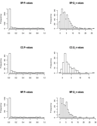
We applied the proposed two sample test with 5% significant level to test each of the gene-sets in conjunction with the Bonferroni correction to

control the family-wise error rate at 0.05 level. It was found that there were

259 gene-sets declared significant in the BP group, 110 in the MF group and 53 in the CC group. Figure 1 displays the histograms of the P-values and the

values of test statistic Qn for the three gene-categories. It shows a strong

non-uniform distribution of the P-values with a large number of P-values

clustered near 0. At the same time, theQn-value plots indicate the average

Qn-values were much larger than zero. These explain the large number of

significant gene-sets detected by the proposed test.

The number of the differentially expressed gene-sets may seem to be high. This was mainly due to overlapping gene-sets. To appreciate this point, we

computed for each (say i-th) significant gene-set, the number of other

sig-nificant gene-sets which overlapped with it, saybi; and obtained the average

of_{bi}and their standard deviation. The average number of overlaps

(stan-dard deviation) for BP group was 198.9(51.3), 55.6 (25.2) for MF, and 41.6 (9.5) for CC. These number are indeed very high and reveals the gene-sets and their P-values were highly dependent.

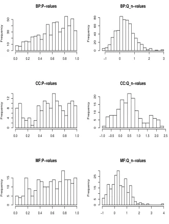
Finally, we carried out back-testing for the same hypothesis by randomly splitting the 42 BRC/ABL class into two sub-class of equal sample size and

testing for mean differences. This set-up led to the situation ofH0. Figures 2

reports the P-values andQn-values for the three Gene Ontology groups. We

note that the distributions of the P-values were much closer to the uniform

distribution than Figure 1. It is observed that the histograms of Qn-values

were centered close to zero and were much closer to the normal distribution than their counterparts in Figure 1, which were reassuring.

5. Simulation Studies. In this section, we report results from simula-tion studies which were designed to evaluate the performance of the proposed two sample test for high dimensional data. For comparison, we also con-ducted the test proposed by Bai and Saranadasa (1996) (BS test), and two tests based on multiple comparison procedures by employing the Bonferroni and the FDR control ( Benjamini and Hochberg, 1995). Both procedures

control the family-wise error rate at a level of significanceα which coincides

mul-tiple comparison procedures, we conducted univariate two samplet-tests for

univariate hypothesesH0l:µ1l =µ2l versus µ1l=µ2l forl= 1,2,· · · , p.

Two simulation models for Xij were considered. One had a moving

av-erage structure that allows a general dependent structure; the other could allocate the the alternative hypotheses sparsely which enable us to evaluate the performance of the tests under sparsity.

5.1. Moving Average Model. The first simulation model has the following moving average structure:

Xijk =ρ1Zijk+ρ2Zijk+1+· · ·+ρpZijk+p−1+µij

for i = 1 and 2, j = 1,2,_{· · ·}, ni and k = 1,2,· · · , p, where {Zijk} were

respectively IID random variables. We considered two distributions for the

innovations _{Zijk}. One was a centralized Gamma(4,1) so that it has zero

mean, and the other wasN(0,1).

For each distribution of _{Zijk}, we considered two configurations of

de-pendence among components of Xij. One had weaker dependence with

ρl = 0 for l > 3. This prescribed a “two dependence” moving average

structure where Xijk1 and Xijk2 are dependent only if |k1 −k2| ≤ 2. The

{ρl}3l=1 were generated independently fromU(2,3), which were ρ1 = 2.883,

ρ2 = 2.794 and ρ3 = 2.849 and were kept fixed throughout the

simula-tion. The second configuration had allρl’s generated fromU(2,3), and were

again keep fixed throughout the simulation. We call this the “full dependence case”. The above dependence structures assigned equal covariance matrices

Σ1= Σ2 = Σ and allows a meaningful comparison with BS test.

Without loss of generality, we fixedµ1= 0 and choseµ2 in the same

fash-ion as Benjamini and Hochberg (1995). Specifically, the percentage of true

null hypothesesµ1l=µ2lforl= 1,· · · , pwere chosen to be 0%,25%,50%,75%,

95% and 99% and 100% , respectively. Experimenting 95% and 99% was

de-signed to gain information on the performance of the test when µ1l = µ2l

were sparse. It provided empirical checks on the potential concerns on the power of the simultaneous high dimensional test as made at the end of Sec-tion 3. At each percentage level of true null, three patterns of allocaSec-tion

were considered for the non-zero µ2l in µ2 = (µ21,· · · , µ2p)′: (i) the equal

allocation where all the non-zeroµ2lwere equal; (ii) linearly increasing and

(iii) linearly decreasing allocations as specified in Benjamini and Hochberg

(1995). To make the power comparable among the configurations ofH1, we

set η =: _||µ1−µ2||2/tr(Σ2) = 0.1 throughout the simulation. We chose

p= 500 and 1000 and n= [20 log(p)] = 124 and 138, respectively.

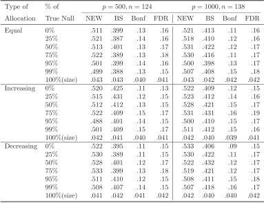
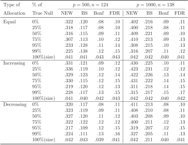
rate or FDR based on 5000 simulations. The results for the Normal innova-tions had similar pattern, and are not reported here. The simulation results in Tables 1 and 2 can be summarized as follows. The proposed test was much more powerful than Bai-Saranadasa test for all cases considered in the simulation, while maintaining a reasonable size approximation to the nominal 5% level. Both the proposed test and Bai-Saranadasa test were more powerful than the two tests based on the multiple univariate testing using the Bonferroni and FDR procedures. This is a little expected as both the proposed and Bai-Saranadasa test are designed to test for the entire

p-dimensional hypotheses while the multiple testing procedures are targeted

at the individual univariate hypothesis. What is surprising is that when the percentage of true null was high at 95% and 99%, the proposed test still were much more powerful than the two multiple testing procedures for all

three allocations of the non-zero components in µ2. It is observed that the

sparsity (95% and 99% true null) does reduce the power of the proposed test a little. However, the proposed test still enjoyed good power, especially comparing with the other three tests. We also observe that when there was more dependence among multivariate components of the data vectors in the full dependence model, there was a drop in the power for each of the test. The power of the tests based on the Bonferroni and FDR procedures were alarmingly low and were only slightly larger than the nominal significance level.

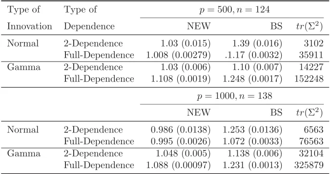
We also collected information on the quality oftr(Σ2_{) estimation. Table 3}

reports empirical averages and standard deviation oftr(Σ2_)/tr(Σ2_{). It shows}

that the proposed estimator fortr(Σ2_{) has much smaller bias and standard}

deviation than those proposed in Bai and Saranadasa (1996) in all cases, and provides an empirical verification for Theorem 2.

5.2. Sparse Model. An examination of the previous simulation setting

reveals that the strength of the “signals” µ2l −µ1l corresponding to the

alternative hypotheses were low relative to the level of noise (variance), which may not be a favorable situation for the two tests based on multiple univariate testing. To gain more information on the performance of the tests under sparsity, we considered the following simulation model such that

X1il =Z1il and X2il =µl+Z2il for l= 1, . . . , p

where _{Z1il, Z2il}p_l=1 are mutually independent N(0,1) random variables,

and the “signals”

µl=ε

for somec_∈(0,1). Hereqis the number of significant alternative hypotheses.

The sparsity of the hypotheses is determined by c: the smaller thec is, the

more sparse the alternative hypotheses withµl= 0. This simulation model

is similar to the one used in Abramovich, Benjamini, Donoho and Johnstone (2006).

According to (3.11), the power of the proposed test has asymptotic power

β(_||µ_||) = Φ

−ξα+

np(c−1/2)_ε2_log(p)

2√2

which indicates that the test has a much reduced power if c < 1/2 with

respect to p. We, therefore, chose p = 1000 and c = 0.25,0.35,0.45 and

0.55 respectively, which led to q = 6,11,22, and 44 respectively. We call

c= 0.25,0.35 and 0.45 the sparse cases.

In order to prevent trivial powers of α or 1 in the simulation, we set

ε= 0.25 for c= 0.25 and 0.45; and ε= 0.15 forc= 0.35 and 0.55. Table 4

summarizes the simulations results based on 500 simulations. It shows that in

the extreme sparse cases ofc= 0.25, the FDR and Bonferroni tests did had

lower power than the proposed test. The power were largely similar among

the three tests for c = 0.35. However, when the sparsity was moderated

to c= 0.45, the proposed test started to surpass the FDR and Bonferroni

procedures. The gap in power performance was further increased whenc=

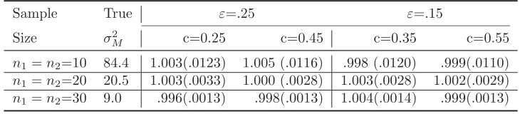
0.55. Table 5 reports the quality of the variance estimation in Table 5, which

shows the proposed variance estimators incurs very little bias and variance

for even very small sample sizes ofn1 =n2 = 10.

6. Technical Details.

6.1. Derivations for E(Tn) and V ar(Tn). As

Tn=

Σn1

i=jX1′iX1j

n1(n1−1)

+ Σ

n2

i=jX2′iX2j

n2(n2−1) −

2Σ

n1

i=1Σn

2

j=1X1′iX2j

n1n2

,

it is straight forward to show thatE(Tn) =µ1′µ1+µ′2µ2−2µ′1µ2 =||µ1−µ2||2.

LetP1=

Σn1

i=jX

′

1iX1j

n1(n1−1) , P2 =

Σn2

i=jX

′

2iX2j

n2(n2−1) andP3 =−2

Σn1

i=1Σ

n2

j=1X

′

1iX2j

n1n2 . It can

be shown that

V ar(P1) = 2 n1(n1−1)

tr(Σ2₁) +4µ

′

1Σ1µ1 n1

,

V ar(P2) = 2 n2(n2−1)

tr(Σ2₂) + 4µ

′

2Σ2µ2 n2

V ar(P3) = 4 n1n2

tr(Σ1Σ2) +

4µ′

2Σ1µ2 n1

+4µ

′

1Σ2µ1 n2

.

Because two samples are independent,Cov(P1, P2) = 0.Also,

Cov(P1, P3) =−

4µ′

1Σ1µ2 n1

and Cov(P2, P3) =−

4µ′

1Σ2µ2 n2

.

In summary,

V ar(Tn) =

2 n1(n1−1)

tr(Σ2₁) + 2

n2(n2−1)

tr(Σ2₂) + 4 n1n2

tr(Σ1Σ2)

+ 4

n1

(µ1−µ2)′Σ1(µ1−µ2) +

4 n2

(µ1−µ2)′Σ2(µ1−µ2).

Thus, underH0

V ar(Tn) =σn21=: 2 n1(n1−1)

tr(Σ2₁) + 2

n2(n2−1)

tr(Σ2₂) + 4 n1n2

tr(Σ1Σ2).

UnderH1 :µ1=µ2, with (3.4),

V ar(Tn) =σn21{1 +o(1)};

and with (3.5),

V ar(Tn) =σn22{1 +o(1)}

whereσn2 = _n41(µ1−µ2)

′_Σ1(µ

1−µ2) + _n42(µ1−µ2)

′_Σ2(µ

1−µ2).

6.2. Asymptotic Normality of Tn. We note that Tn=Tn1+Tn2 where

Tn1 =

Σn1

i=j(X1i−µ1)′(X1j −µ1) n1(n1−1)

+Σ

n2

i=j(X2i−µ2)′(X2j −µ2) n2(n2−1)

−2Σ

n1

i=1Σn

2

j=1(X1i−µ1)′(X2j −µ2) n1n2

. (6.1)

and

Tn2 = Σ

n1

i=1(X1i−µ1)′(µ1−2µ2) n1

+ Σ

n2

i=1(X2i−µ2)′(µ2−2µ1) n2

+µ′₁µ1+µ′2µ2−2µ′1µ2.

It is easy to show thatE(Tn1) = 0 andE(Tn2) =||µ1−µ2||2, and

V ar(Tn2)

Letσ_n2 be the leading order V ar(Tn) as given in the subsection 6.1.

Under (3.4), as

V ar(Tn2− ||µ1−µ2|| 2

σn1

) =o(1),

(6.2) Tn− ||µ1−µ2||

2

V ar(Tn)

= Tn1

σn1

+op(1).

Under (3.5),

(6.3) Tn− ||µ1−µ2||

2

V ar(Tn)

= Tn2− ||µ1−µ2||

2

σn2

+op(1).

AsTn2are independent sample averages, its asymptotic normality is

read-ily attainable as showed later. The main task of the proof is for the case

un-der (3.4) whenTn1 is the contributor of the asymptotic distribution. From

(6.1), in the derivation for the asymptotic normality ofTn1, we can assume

without loss of generality µ1=µ2= 0.

LetYi =X1i fori= 1,· · · , n1 and Yj+n1 =X2j forj = 1,· · · , n2, and for i=j

φij =

⎧ ⎪ ⎪ ⎨ ⎪ ⎪ ⎩

n−₁1(n1−1)−1Yi′Yj, ifi, j∈ {1,2,· · · , n1},

−n−₁1n−₂1Y_i′Yj, ifi∈ {1,2,· · · , n1} and j∈ {n1+ 1,· · · , n1+n2}, n−₂1(n2−1)−1Yi′Yj, ifi, j∈ {n1+ 1,· · · , n1+n2}.

DefineVnj =ij=1−1φij forj= 2,3,· · · , n1+n2,Snm=mj=2Vnj andFnm=

σ_{Y1, Y2,· · ·, Ym}which is theσalgebra generated by{Y1, Y2,· · · , Ym}.Now

Tn= 2

n1+n2

j=2 Vnj.

Lemma 1:For eachn,_{Snm,Fnm}nm=1 is the sequence of zero mean and a square integrable martingale.

Proof. It’s obvious that _Fnj−1 ⊆ Fnj, for any 1≤j ≤n and Snm is of

zero mean and square integrable. We only need to showE(Snq|Fnm) =Snm

for any q_≥m. We note that

Ifj_≤m_≤n, thenE(Vnj|Fnm) = Σij=1−1E(φij|Fnm) = Σij=1−1φij =Vnj.

Ifj > m, thenE(φij|Fnm) =E(Yi′Yj|Fnm).

Ifi > m, as Yi and Yj are both independent of Fnm,

Ifi_≤m, E(φij|Fn,m) =E(Yi′Yj|Fn,m) =YiE(Yj′) = 0.Hence,

E(Vnj|Fn,m) = 0.

In summary, for q > m, E(Snq|Fnm) = Σqj=1E(Vnj|Fnm) = Σmj=1Vnj =

Snm. This completes the proof of the lemma.

Lemma 2:Under Condition (3.4),

Σn1+n2

j=2 E[Vnj2|Fn,j−1]→P 1₄σT2n.

Proof. Note that

E(V_nj2_|Fnj−1) =E{(

j−1

i=1

Y_i′Yj)2|Fnj−1}=E(

j−1

i1,i2=1 Y_i′1YjY

′

jYi2|Fnj−1)

=

j−1

i1,i2=1

Y_i′1E(YjY

′

j|Fnj−1)Yi2 =

j−1

i1,i2=1

Y_i′1E(YjY

′

j)Yi2

=

j−1

i1,i2=1 Y_i′1

˜

Σj

˜

nj(˜nj−1)

Yi2

where ˜Σj = Σ1,n˜j = n1, for j ∈ [1, n1] and ˜Σj = Σ2, ˜nj = n2, if j ∈

[n1+ 1, n1+n2].

Define

ηn=

n1+n2

j=2

E(V_nj2_|Fnj−1)

Then,

E(ηn) =

tr(Σ2₁)

2n1(n1−1)

+ tr(Σ

2 2)

2n2(n2−1)

+ tr(Σ1Σ2)

(n1−1)(n2−1)

= 1₄σ_T2_n.

(6.4)

Now consider

E(η_n2) = E_{

n1+n2

j=2

j−1

i1,i2=1 Y_i′1

˜

Σj

˜

nj(˜nj−1)

Yi2}

2

= E_{2

n1+n2

2≤j1<j2

j1−1

i1,i2=1

j2−1

i3,i4=1 Y_i′1

˜

Σj1

˜

nj1(˜nj1−1) Yi2Y

′

i3

˜

Σj2

˜

nj2(˜nj2−1) Yi4

(6.5)

+

n1+n2

j=2

j−1

i1,i2=1

j−1

i3,i4=1 Y_i′1

˜

Σj

˜

nj(˜nj−1)

Yi2Y

′

i3

˜

Σj

˜

nj(˜nj−1)

Yi4}

where

A =

n1+n2

2≤j1<j2

j1−1

i1,i2=1

j2−1

i3,i4=1 Y_i′1

˜

Σj1

˜

nj1(˜nj1 −1) Yi2Y

′

i3

˜

Σj2

˜

nj2(˜nj2 −1) Yi4,

B =

n1+n2

j=2

j−1

i1,i2=1

j−1

i3,i4=1 Y′

i1

˜

Σj

˜

nj(˜nj −1)

Yi2Y

′

i3

˜

Σj

˜

nj(˜nj −1)

Yi4.

(6.6)

Derivations given in Chen and Qin (2008) show

2E(A) =

_tr2_(Σ2 1)

4n2

1(n1−1)2

+ tr

2_(Σ2 2)

4n2

2(n2−1)2

+ tr(Σ

2

1)tr(Σ1Σ2) n2

1(n1−1)(n2−1)

+ tr(Σ

2

2)tr(Σ1Σ2)

(n1−1)n2(n2−1)

+ tr

2_(Σ 2Σ1) n1n2(n1−1)(n2−1)

+ tr(Σ

2

1)tr(Σ22)

2n1(n1−1)n2(n2−1)

{+o(1)_}.

andE(B) =o(σ2

Tn). Hence, from (6.5) and (6.6),

E(η_n2) =

_tr2_(Σ2 1)

4n2

1(n1−1)2

+ tr

2_(Σ2 2)

4n2

2(n2−1)2

+ tr(Σ

2

1)tr(Σ1Σ2)

n2

1(n1−1)(n2−1) +

+ tr(Σ

2

2)tr(Σ1Σ2)

(n1−1)n2(n2−1)

+ tr

2_(Σ 2Σ1) n1n2(n1−1)(n2−1)

+ tr(Σ

2

1)tr(Σ22)

2n1(n1−1)n2(n2−1)

+o(σ4_Tn).

(6.7)

Based on (6.4) and (6.7),

V ar(ηn) =E(ηn2)−E2(ηn) =o(σT4n).

(6.8)

Combine (6.4) and (6.8), we have

σ−_Tn2E

Σn1+n2

j=1 E(Vnj2|Fn,j−1)

=σ_T−_n2E(ηn) = 1₄, and

σ−_Tn4V ar

Σn1+n2

j=1 E(Vnj2|Fn,j−1)

=σ−_Tn4V ar(ηn) =o(1).

This completes the proof of Lemma 2.

Lemma 3Under the condition (3.4),

n1+n2

j=2 σ_T−2

nE{V

2

njI(|Vnj|> ǫσTn)|Fnj−1}

p

Proof. We note that

n1+n2

j=2

σ_T−_n2E_{V_nj2I(_|Vnj|> ǫσTn)|Fnj−1} ≤σ

−q Tnǫ

2−q n1+n2

j=1

E(V_njq_|Fnj−1);

for someq >2. By choosingq= 4, the conclusion of the lemma is true if we

can show

E_{

n1+n2

j=2

E(V_nj4_|Fnj−1)}=o(σ4Tn).

(6.9)

We notice that

E_{

n1+n2

j=2

E(V_nj4_|Fnj−1)}=

n1+n2

j=1

E(V_nj4) =

n1+n2

j=1 E(

j−1

i=1 Y_i′Yj)4

=

n1+n2

j=2

j−1

i1,i2,i3,i4

E(Y_i′1YjY

′

i2YjY

′

i3YjY

′

i4Yj).

The last term can be decomposed as 3Q+P where

Q=

n1+n2

j=2

j−1

s=t

E(Y_j′YsYs′YjYj′YtYt′Yj)

and P = Σn1+n2

j=2 Σ

j−1

s=1E(Ys′Yj)4. Now (6.9) is true if 3Q+P =o(σT4n).

Note that

Q=

n1+n2

j=2

j−1

s=t

E_{tr(YjYj′YtYt′YjYj′YsYs′)}

=O(n−4)_{

n1

j=2

j−1

s=t

E(Y_j′Σ1YjYj′Σ1Yj) + n1+n2

j=n1+1

j−1

s=t

E(Y_j′ΣtYjYj′ΣsYj)}=o(σT4n).

The last equation follows the similar procedure in Lemma 2 under (3.4).

It remains to showP = Σn1+n2

j=2 Σj

−1

s=1E(Ys′Yj)4=o(σT4n). Note that

P =

n1+n2

j=2

j−1

s=1

E(Y_s′Yj)4 = n1

j=2

j−1

s=1

E(Y_s′Yj)4+ n1+n2

j=n1+1

j−1

s=1

E(Y_s′Yj)4

= O(n−8_){

n1

j=2

j−1

s=1 E(X′

1sX1j)4+ n1+n2

j=n1+1

n1

s=1 E(X′

1sX2j−n1)

4

+

n1+n2

j=n1+1

j−1

s=n1+1

E(X₂′_s−n1X2j−n1)

4_}

where P1 = nj=21

j−1

s=1E(X1′sX1j)4, P2 = nj=1+nn1+12 n1

s=1E(X1′sX2j−n1)

4

and

P3 =

n1+n2

j=n1+1

j−1

s=n1+1

E(X₂′_s−n1X2j−n1)

4_.

Let us consider E(X′

1sX2j−n1)

4_{. Define Γ}′

1Γ2 =: (vij)m×m and note the

following facts which will be used repeatedly in the rest of the appendix,

m

i,j=1 v4_{ij ≤}(

m

i,j=1

v_ij2)2 =tr2(Γ′₁Γ2Γ′2Γ1) =tr2(Σ2Σ1),

m

i=1

m

j1=j2

(v_ij21v

2

ij2)≤(

m

i,j=1

v_ij2)2 =tr2(Σ2Σ1),

m

i1=i2

m

j1=j2

vi1j1vi1j2vi2j1vi2j2 ≤

m

i1=i2

v(2)_i1i2v(2)_{i1i2 ≤}

m

i1i2=1

v_i(2)_1i2v_i(2)_1i2,

m

i1i2=1

v(2)_i1i2v(2)_i1i2 =

m

i1=1

v(4)_i1i1 =tr(Γ′₁Σ2Γ1Γ′1Σ2Γ1) =tr(Σ2Σ1)2,

where Γ′

1Σ′2Γ1= (v(2)ij ) and (Γ′1Σ2Γ1)2 = (vij(4))m×m.

From (3.1),

E(X₁′_sX2j−n1)

4₌m

i=1

m

j′₌₁

(3 + ∆)2v4_ij′+

m

i=1

(3 + ∆)

m

j1=j2 v2_ij1v

2

ij2

+

m

j′₌₁

(3 + ∆)

m

i1=i2 v2_i1jv

2

i2j + 9

m

i1=i2

m

j1=j2

vi1j1vi1j2vi2j1vi2j2

=O_{tr2(Σ2Σ1)_}+O_{tr(Σ2Σ1)2_}.

Then we conclude

O(n−8)P2=

n1+n2

j=n1+1

n1

s=1

O_{tr2(Σ2Σ1)}+O{tr(Σ2Σ1)2}

=O(n−5)

O_{tr2(Σ2Σ1)}+O{tr(Σ2Σ1)2}

=o(σ4_Tn).

We can also prove thatO(n−8_)P

1 =o(σT4n) andO(n

−8_)P

3 =o(σ4Tn) by going

6.3. Proof of Theorem 1.

Proof. We note equations (6.2) and (6.3) under conditions (3.4) and

(3.5) respectively. Based on Corollary 3.1 of Hall and Heyde (1980), Lemma

1, Lemma 2 and Lemma 3, it can be concluded thatTn1/σn1 →d N(0,1). This

implies the desired asymptotic normality ofTn under (3.4). Under (3.5), as

Tn2 is the sum of two independent averages, its asymptotic normality can be

attained by following the standard means. Hence the theorem is proved.

6.4. Proof of Theorem 2.

Proof. We only present the proof for the ratio consistency of tr(Σ2 1) as the proofs of the other two follow the same route. We want to show

(6.10) E_{tr(Σ2

1)}=tr(Σ21){1 +o(1)}and V ar{tr(Σ21)}=o{tr2(Σ21)}.

For notation simplicity, we denote X1j as Xj and Σ1 as Σ, since we are

effectively in a one sample situation. Note that

tr(Σ2₎

= _{n(n₋1)_}−1tr[

n

j=k

(Xj −µ)(Xj−µ)′(Xk−µ)(Xk−µ)′

−2( ¯X(j,k)−µ)(Xj −µ)′(Xk−µ)(Xk−µ)′

+

n

j=k

2(Xj−µ)µ′(Xk−µ)(Xk−µ)′−2( ¯X(j,k)−µ)µ′(Xk−µ)(Xk−µ)′

+

n

j=k

( ¯X_(j,k)−µ)(Xj−µ)′( ¯X(j,k)−µ)(Xk−µ)′

−

n

j=k

2(Xj −µ)µ′( ¯X(j,k)−µ)(Xk−µ)′

−2( ¯X(j,k)−µ)µ′( ¯X(j,k)−µ)(Xk−µ)′

+

n

j=k

(Xj −µ)µ′(Xk−µ)µ′−2( ¯X(j,k)−µ)µ′(Xk−µ)µ′

+

n

j=k

( ¯X(j,k)−µ)µ′( ¯X(j,k)−µ)µ′]

=: 10

l=1

It is easy to show that E_{tr(A1)}=tr(Σ2), E{tr(Ai)}= 0 fori= 2,· · ·,9

and E_{tr(A10)} = µ′Σµ/(n−2) = o{tr(Σ2)}. The last equation is based

on (3.4). This leads to the first part of (6.10). Sincetr(A10) is non-negative

and E_{tr(A10)} = o{tr(Σ2)}, we have tr(A10) = op{tr(Σ2)}. However, to

establish the orders of other terms, we need to deriveV ar_{tr(Ai)}. We shall

only show V ar_{tr(A1)} here. Derivations for other V ar{tr(Ai)} are given

in Chen and Qin (2008). Note that

V ar_{tr(A1)_}+tr2(Σ2)

=E[ 1

n(n₋1)tr

n

j=k

(Xj −µ)(Xj−µ)′(Xk−µ)(Xk−µ)′]2

= 1

n2_(n−1)2E[tr

n

j1=k1

(Xj1 −µ)(Xj1 −µ)

′

(Xk1 −µ)(Xk1 −µ)

′

×tr

n

j2=k2

(Xj2−µ)(Xj2 −µ)

′_(X

k2 −µ)(Xk2 −µ)

′_].

It can be shown, by considering the possible combinations of the subscripts j1, k1, j2 and k2, that

V ar_{tr(A1)} = {n(n−1)}−1E (X1−µ)′(X2−µ)4+

4(n₋2)

n(n₋1)E

(X1−µ)′Σ(X1−µ)

2

+o_{tr2(Σ2)_}

=: 2

n(n₋1)B11+

4(n₋2)

n(n₋1)B12+o{tr

2_(Σ2_)}, (6.11)

where

B11=E(Z1′Γ′ΓZ2)4 =E(

m

s,t=1

z1sνstz2t)4

=E(

m

s1,s2,s3,s4,t1,t2,t3,t4=1

νs1t1νs2t2νs3t3νs4t4z1s1z1s2z1s3z1s4z2t1z2t2z2t3z2t4)

and

B12=E(Z1′Γ′ΓΓ′ΓZ1)2 =E(

m

s,t=1

z1sustz1t)2

=E(

m

s1,s2,t1,t2=1

Hereνst and ust are respectively the (s, t) element of Γ′Γ and Γ′ΣΓ.

Since tr2_(Σ2_{) = (}m

s,t=1νst2)2 = sm1,s2,t1,t2=1ν

2

s1t1ν

2

s2t2 and tr(Σ

4_{) =}

m t1,t2=1u

2

t1t2. It can be shown that A11 ≤ c tr

2_(Σ2_{) for a finite positive}

number c and hence _{n(n₋1)_}−1_B

11 = o{tr2(Σ2)}. It may also be shown

that

B12= 2

m

s,t=1 u2_st+

m

s,t=1

ussutt+ ∆ m

s=1 u2_ss

= 2tr(Σ4) +tr2(Σ2) + ∆

m

s=1 u2_ss

≤(2 + ∆)tr(Σ4) +tr2(Σ2).

Therefore, from (6.11)

V ar_{tr(A1)} ≤ 2 n(n₋1)ctr

2_(Σ2_{) +} 4(n−2) n(n₋1)

(2 + ∆)tr(Σ4) +tr2(Σ2)

+(n−2)(n−3)

n(n₋1) tr

2_(Σ2₎

−tr2(Σ2)

=o_{tr2(Σ2)_}.

This completes the proof.

Acknowledgements. We are grateful to two reviewers for valuable comments and suggestions which have improved the presentation of the pa-per. We also thank Dan Nettleton and Peng Liu for useful discussions.

References.

[1] Anderson, T. W.(2003).An Introduction to Multivariate Statistical Analysis. Wiley.

[2] Abramovich, F., Benjamini, Y., Donoho, D. L. and Johnstone, I. M.(2006). Adaptive to unknown sparsity in controlling the false discovery rate. The Annals of Statistics 34_{, 584-653.}

[3] Bai, Z. and Saranadasa, H.(1996). Effect of high dimension: by an example of a two sample problem.Statistica Sinica 6_311–329.

[4] Barry, W., Nobel, A. and Wright, F.(2005). Significance analysis of functional categories in gene expression studies: A structured permutation approach. Bioinfor-matics21_1943-1949.

[6] Benjamini, Y. and Yekutieli, D.(2001). The control of the false discovery rate in multiple testing under dependency.The Annals of Statistics 29_{, 1165–1188.}

[7] Chen, S. X. and Qin, Y.-L.(2008).A Two Sample Test For High Dimensional Data With Applications To Gene-set Testing. Research Report, Department of Statistics, Iowa State University.

[8] Chiaretti, S., Li, X.C., Gentleman, R., Vitale, A., Vignetti, M., Mandelli, F., Ritz,J. and Foa, R. (2004) Gene expression profile of adult T-cell acute lymphocytic leukemia identifies distinct subsets of patients with different response to therapy and survival. Blood 103_{, No. 7, 2771–2778.}

[9] Dudoit, S., Keles, S. and van der Laan, M.(2006). Multiple tests of association with biological annotation metadata. Manuscript.

[10] Efron, B. and Tibshirani, R.(2007). On testing the significance of sets of genes. The Annals of Applied Statistics,1_{, 107-129.}

[11] Fan, J., Hall, P. and Yao, Q.(2007). To how many simultaneous hypothesis tests can normal, student’s t or bootstrap calibration be applied. Journal of the American Statistical Association,102_{, 1282-1288.}

[12] Fan, J., Peng, H. and Huang, T. (2005). Semilinear high-dimensional model for normalization of microarray data: a theoretical analysis and partial consistency. Journal of the American Statistical Association,100_{, 781-796.}

[13] Gentleman, R., Irizarry, R.A., Carey, V.J., Dudoit, S. and Huber, W. c(2005). Bioinformatics and Computational Biology Solutions Using R and Biocon-ductor, Springer.

[14] Hall, P. and Heyde, C.(1980). Martingale Limit Theory and Applications, Academic Press, New York.

[15] Huang, J., Wang, D. and Zhang, C. (2005). A two-way semilinear model for normalization and analysis of cDNA microarray data. Journal of the American Statistical Association100_814–829.

[16] Kosorok, M. and Ma, S. (2007). Marginal asymptotics for the ”large p, small n” paradigm: with applications to microarray data. The Annals of Statistics, 35_,

1456-1486.

[17] Ledoit, O. and Wolf, M.(2002). Some hypothesis tests for the covariance matrix when the dimension is large compare to the sample size. The Annals of Statistics,

30_{, 1081-1102.}

[18] Newton, M., Quintana, F., Den Boon, J., Sengupta, S. and Ahlquist, P. (2007). Random-set methods identify distinct aspects of the enrichment signal in gene-set analysis. The Annals of Applied Statistics,1_{, 85-106.}

[19] Portnoy, S.(1986). On the central limit theorem inRp _whenp

Theory and Related Fields,73_{, 571-583.}

[20] Recknor, J., Nettleton, D. and Reecy, J.(2007). Identification of differentially expressed gene categories in microarray studies using nonparametric multivariate analysis. Bioinformatics, to appear.

[21] Schott, J. R. (2005). Testing for complete independence in high dimensions. Biometrika,92_{, 951-956.}

[22] Storey, J., Taylor, J. and Siegmund, D. (2004). Strong control, conservative point estimation and simultaneous conservative consistency of false discovery rates: a unified approach. Journal of the Royal Statistical Society series B,66_{, 187–205.}

[23] Tracy, C. and Widom, H.(1996). On orthogonal and symplectic matrix ensembles. Communications in Mathematical Physics 177_{, 727–754.}

[24] van der Laan, M. and Bryan, J. (2001). Gene expression analysis with the parametric bootstrap. Biostatistics 2_{, 445–461.}

BP:P−values

Frequency

0.0 0.2 0.4 0.6 0.8 1.0

0

100

300

BP:Q_n values

Frequency

0 5 10 15 20 25

0

2

04

06

08

0

CC:P−values

Frequency

0.0 0.2 0.4 0.6 0.8 1.0

0

2

04

06

08

0

CC:Q_n values

Frequency

0 5 10 15

01

0

2

0

3

0

4

0

MF:P−values

Frequency

0.0 0.2 0.4 0.6 0.8 1.0

0

50

100

150

MF:Q_n values

Frequency

0 5 10 15 20 25 30

01

0

2

0

3

0

Fig 1. Two sample tests for differentially expressed gene-sets between BCR/ABL and NEG class ALL: Histograms of P-values (left panels) andQnvalues (right panels) for BP, CC

BP:P−values

Frequency

0.0 0.2 0.4 0.6 0.8 1.0

0

1

03

05

0

BP:Q_n−values

Frequency

−1 0 1 2 3

0

2

04

06

08

0

CC:P−values

Frequency

0.0 0.2 0.4 0.6 0.8 1.0

048

1

2

CC:Q_n−values

Frequency

−1.0 −0.5 0.0 0.5 1.0 1.5 2.0 2.5

0

5

10

15

20

MF:P−values

Frequency

0.0 0.2 0.4 0.6 0.8 1.0

0

5

10

15

MF:Q_n−values

Frequency

−1 0 1 2 3 4

0

5

15

25

Fig 2. Back-testing round 2 for differentially expressed gene-sets between two randomly assigned BCR/ABL groups: Histograms of P-values (left panels) and Qn values (right

Table 1. Empirical Power and Size for the 2-Dependence Model with Gamma Innovation

Table 2. Empirical Power and Size for the Full-Dependence Model with Gamma Innovation

Table 3. Empirical averages of tr(Σ2_)/tr(Σ2_{) with standard deviations in} the parentheses.

Type of Type of p= 500, n= 124

Innovation Dependence NEW BS tr(Σ2₎

Normal 2-Dependence 1.03 (0.015) 1.39 (0.016) 3102 Full-Dependence 1.008 (0.00279) .1.17 (0.0032) 35911 Gamma 2-Dependence 1.03 (0.006) 1.10 (0.007) 14227 Full-Dependence 1.108 (0.0019) 1.248 (0.0017) 152248

p= 1000, n= 138

NEW BS tr(Σ2₎

Table 4. Empirical Power and Size for the Sparse Model.

Sample ε=.25 ε=.15

Size c=.25 c=.45 c=.35 c=.55

(n₁=n₂) Methods Power Size Power Size Power Size Power Size

10 FDR .084 .056 .180 .040 .044 .034 .066 .034 Bonf .084 .056 .170 .040 .044 .034 .062 .032 New .100 .046 .546 .056 .072 .064 .344 .064 20 FDR .380 .042 .855 .044 .096 .036 .326 .058 Bonf .368 .038 .806 .044 .092 .034 .308 .056 New .238 .052 .976 .042 .106 .052 .852 .046 30 FDR .864 .042 1 .060 .236 .048 .710 .038 Bonfe .842 .038 .996 .060 .232 .048 .660 .038 New .408 .050 .998 .058 .220 .054 .988 .042

Table 5. Average ratios of σ2_M/σ_M2 and their Standard Deviation (in parenthesis) for the Sparse Model

Sample True ε=.25 ε=.15

Size σ2

M c=0.25 c=0.45 c=0.35 c=0.55

n1=n2=10 84.4 1.003(.0123) 1.005 (.0116) .998 (.0120) .999(.0110)

n1=n2=20 20.5 1.003(.0033) 1.000 (.0028) 1.003(.0028) 1.002(.0029)

n1=n2=30 9.0 .996(.0013) .998(.0013) 1.004(.0014) .999(.0013)

Department of Statistics Iowa State University Ames, Iowa 50011-1210;

and Guanghua School of Management, Peking University, Beijing 100871, China E-mail:[email protected]

Department of Statistics Iowa State University Ames, Iowa 50011-1210;