267
*The views expressed in this paper are not necessarily those held by the Central Bank of Ireland and are the personal responsibility of the authors.
The Expectations Hypothesis of the Term
Structure: The Case of Ireland*
KEITH CUTHBERTSON
Management School, Imperial College London
and
DON BREDIN
Central Bank of Ireland
Abstract:Using a number of short-term maturities and monthly data, 1984-1997, we provide a
number of tests of the expectations hypothesis (EH) of the term structure. The paper draws on co-integration techniques and the methodological approach of Campbell and Shiller (1987,1991). On balance our results lend support to the EH and are broadly consistent with recent findings for the UK, but are in sharp contrast to those for the US.
I INTRODUCTION
T
he expectations hypothesis (EH) of the term structure implies that the yield spread between the long rate and short rate is an optimal predictor of future changes in short rates over the life of the “long bond”.changes in short rates are not often closely correlated with the long-short spread (Campbell and Shiller, 1991).
Kugler (1988) using US, German and Swiss monthly data on one and three month Euromarket deposit rates found support for the EH only on German data (for the period of March 1974 to August 1986). Similarly, Engsted (1994) using Danish money market rates and (Engsted and Tanggaard, 1994) for longer maturity bonds find considerable support for the EH when the variation in interest rates is relatively large, such as in the post-1992 ERM “crisis period”. This is to be expected following the analysis of Mankiw and Miron (1986), for if interest rate stabilisation results in random walk behaviour for short rates, then the expected change in short rates is zero and the spread has no predictive power for future short rates (see also Rudebusch, 1995).
Using the Campbell-Shiller VAR methodology on data at the short end of the maturity spectrum (i.e. up to one year) Cuthbertson (1996a) finds reasonable support for the EH on UK data. This is in contrast to Taylor (1992) who uses maturities of 5, 10 and 15 years and finds strongly against the EH (see also MacDonald and Speight, 1991). To our knowledge, the only related paper using Irish data, is that of Hurley (1990).1 Using a number of interest rate combinations for the period 1979 to 1989, Hurley (1990) finds little evidence to support the EH, in that the spread does not forecast future changes in short rates. However, as noted by the author, the study suffers a number of drawbacks. First, the data used in the study are yields taken from the Central Bank Bulletin and so are not continuously compounded spot rates as required by (linear) tests of the EH. Second, the author uses OLS estimation, which is inappropriate, given the inclusion of overlapping observations.
The main aim of this paper is to present evidence on the behaviour of the term structure of Irish interest rates at the short end of the maturity spectrum. The paper applies co-integration techniques and the methodological approach of Campbell and Shiller (1987,1991).2 To our knowledge the expectations hypothesis (EH) using the VAR approach has not been examined using Irish data. We test parameter restrictions on the VAR models using a high quality data set. By using spot rates based on quoted discount rates we avoid having to use an approximation to zero coupon yields and the par yield approximation
1. McGettigan (1995) drawing on the approach of McCulloch (1971, 1975) “fits” yield curves to Irish rates using discount functions but does not test the EH, as is done in this paper . As noted by McGettigan, a similar “curve fitting” approach was used by Breen and Keogh (1990). Breen (1991) in his comment on Joyce (1991) also draws the distinction between “fitting” yield curves and explicit tests of the EH.
which are required when analysing coupon paying bonds (Shiller, 1979). We also assess the results in comparison to the previous evidence.3
II THE EXPECTATIONS HYPOTHESIS
The expectations hypothesis (EH) of the term structure posits that the return on an n-period bond
Rt
(n) is determined solely by expectations of (current and) future rates on a set of m-period short rates r(m)t (where n > m). Using con-tinuously compounded spot rates the “fundamental term structure” relationship is:
Rt(n)=(1 / k) Etr(m)t+im i=0
k−1
∑ (1)
where k = n/m is an integer and Et is the expectations operator (with information up to and including time t). If there is a time invariant term premium, which is constant for given (n,m) then (1) will also contain a constant term. The intuition behind (1) is easily seen by taking n=3 and m=1. If $1 is invested at the 3-year spot rate, then the certain amount received after 3-years is $(1+Rt)3. Alternatively at t=0, the investor can consider investing $1 at the one-period rate rt and then reinvesting at the one-period rates in years two and three (i.e. rolling over the one-period investment). The latter is a risky strategy and results in expected “dollar” receipts of $(1+rt) (1+Etrt+1) (1+Etrt+2). The EH assumes investors are risk neutral and that the market is efficient, hence in equilibrium (1+Rt)3 = (1+rt) (1+Etrt+1) (1+Etrt+2). Taking logarithms of both sides of the latter expres-sion and noting that ln(1+rt) is the continuously compounded interest rate, we obtain Equation (1) – see Cuthbertson (1996b) for further details.
We can re-arrange (1) in terms of the spread and the change in interest rates (since below we find that these are stationary variables) and (1) can then be seen to imply that the “long-short” spread is an optimal predictor of future changes in short rates, r(m)t :
St(n,m)=Et (1−i / k)∆mr(m)t+im i=1
k−1
∑ =Et
[
PFSt(n,m)]
(2)where St(n,m) = (Rt(n) – rt(m)) is the yield spread. Equation (2) implies that if future short rates are expected to rise, then this will be accompanied by an increase in the spread. To see the intuition behind (2), again consider the case n=3, m=1. Suppose at t=0, investors believe that inflation in years two and three will be higher (than previously anticipated). Then they will revise upwards their forecasts of the one-period rates pertaining to years 2 and 3, that is Etrt+1 and Etrt+2, and hence Et∆rt+1 and Et∆rt+2 will also rise. Therefore, rolling over “one-period” investments will currently give a higher expected return than investing at the 3-year spot rate. Investors will therefore sell 3-year (zero coupon) bonds to invest in one-year bonds, and the price of 3-year bonds will consequently fall. But the latter implies that their yield Rt will rise, as will the spread St = (Rt – rt). Arbitrage ensures that Rt increases until the higher spread just equals the (weighted average of) future expected increases in one-period rates, as summarised in (2). For our simple case, Equation (2) is St = (2/3) Et∆rt+1 + (1/3) Et∆rt+2.
The perfect foresight spread PFStin (2) is simply the (weighted average) of actual future changes in short term rates (which agents are trying to forecast). However, in the literature it is referred to as the “perfect foresight spread” because under the EH, it can also be interpreted as the spread that would ensue if agents had perfect foresight about future movements in interest rates (i.e. made no forecast errors).
A testable implication of Equation (2) is that the spread Granger causes future changes in short rates.4 If (R
t(n), rt(m)) are found to be I(1), then ∆rt(m) is I(0), which from Equation (2) implies that the spread St(n,m) = (R
t(n) – rt(m)) should also be I(0). The latter implies that (Rt(n), rt(m)) should be co-integrated with a co-integrating vector (1, –1).5 If we now add the assumption of rational expectations (RE):
r(m)t+im=Etr(m)t+im+ εt+im (3)
we obtain the following single equation test of the null of the “expectations hypothesis plus rational expectations”, EH + RE:
4. Strictly, failure of Granger causality does not constitute a rejection of the EH, but a failure to confirm it.
PFSt(n,m)= α + βS(n,m)t + γΩt+ ε*t
H0:α = γ =0, β= 1 (4)
ε*t is a moving average error of order (n–m–1) consisting of a weighted sum of future values of εt+im, and Ωt represents the information available to agents at time t, or earlier. Under RE, ε*t is independent of Ωt, and in particular is independent of the yield spread. If there is a constant term premia or if there are differential yet constant transactions costs (between investing “long” and in a series of rolled-over short-term investments) then α≠ 0. Under RE the right hand side variables in Equation (4) are independent of ε*tand hence we do not require IV estimation. However a GMM estimator is employed to correct the covariance matrix for the moving-average error of order (n–m–1) and possible heteroscedasticity (Hansen, 1982; Newey and West, 1987).
III VAR METHODOLOGY
One of the problems in using Equation (2) is the correction needed for overlapping data and it may result in standard errors which are biased in finite samples, with the degree of bias being more severe, the greater the degree of “overlap”. The VAR methodology overcomes the latter defect and also allows forecasts of futures changes in interest rates to be influenced not only by lagged changes in interest rates (as in a single equation framework) but also by the spread, which according to the EH has predictive power for future interest rates (see Equation (2)). More formally, if Zt = (St(n,m), ∆r
t
(m)) is stationary, then there
exists a bivariate Wold representation (Hannan, 1970) which may be approxi-mated by a vector autoregression (VAR) of order p, which in companion form is:
Zt =AZt−1+vt (5)
where A is the matrix of estimated VAR coefficients. Forecasts of future changes in interest rates can be obtained from (5) by noting that Et(Zt+j) = Aj Z
t . However, to test the EH using (2) what we require is a time series of future forecasts of the change in interest rates. This is easily obtained if we create a “selection vector” e2 which has all zero entries except for a single entry of “unity” to “pick out” ∆rt(m) from the Z vector. A forecast of Et∆r
t+j(m) is then given by e2 (A′ jZt). The left hand side of (2) is the spread St(n,m) which is the first entry in the Z vector, so e1’Zt = St(n,m). Substituting Et∆r
e1’= e2’A [I – (m/n)(I – An) (I–Am)–1] (I – A)–1 (6)
We apply Equation (6) on monthly data for (n,m) = (6,3), (6,1), (3,1). The VAR methodology suggests several approaches to testing the EH + RE under weakly rational expectations. The restrictions in (6) can be shown to imply that information at time t other than that contained in St(n,m) should not help to predict
future changes in short rates (i.e. St(n,m) must be an optimal predictor of future changes in short rates). The restrictions on the parameters of the VAR in Equation (6) are tested using a Wald test.6
The forecasts from the VAR of the (weighted average) of future short rates on the right-hand-side of Equation (2) are a complex function of the estimated parameters of the A-matrix of the VAR. This forecast is known as the “theoretical spread”, denoted St(n,m)′ where,
St(n,m)′ = e2’A [I – (m/n)(I – An) (I–Am)–1] (I – A)–1Z
t (7)
Using the VAR estimates of the A-matrix, Equation (7) can be used to give a
time series of the (weighted average) of the forecasts of future changes in interest
rates St(n,m)’. For example, for n=3, m=1 the (weighted) forecast of future changes in one-period interest rates St(3,1)’ = (2/3) Et∆rt+1 + (1/3) Et∆rt+2 and using (7) is easily seen to be given by { (2/3) e2’A + (1/3) e2’A2} Z
t.If the EH is correct then we expect the time series of the theoretical spread St(n,m)’ to move the same as the actual spread St(n,m). Indeed the formal test of the VAR restrictions in (6) are merely testing the hypothesis, H0: St(n,m) = St(n,m)’. Campbell and Shiller (1991) note that formal tests of the VAR restrictions may lead to rejection of the EH even though the deviations from the null are quite small from an economic perspective. They suggest computing the time series forecasts of interest rates in (7) (i.e. the “theoretical spread”), without imposing the VAR restrictions and comparing this with the time series behaviour of the actual spread. If the EH is true then we would expect a graph of the actual spread St(n,m) and the theoretical spread St(n,m)’ to move together and hence for the standard deviation ratio SDR = σ(St(n,m)’)/ σ(St(n,m)), and the correlation coefficient, Corr(St(n,m), St(n,m)’) both to equal unity.7 If σ(S
t(n,m)) > σ(St(n,m)’) then there is “excess volatility”, that is the actual spread is more volatile than the optimal predictor of future short rates.
6. In testing the VAR restrictions we use a GMM correction to the covariance matrix of the VAR system.
7. The standard errors of SDR = σ(St(n,m)′)/ σ(S t
(n,m)) and R ( S t
(n,m), S t
(n,m)′) are non-linear functions
8. We focus on tests of the EH in terms of 3 interest rate combinations; (1,3), (1,6) and (3,6) month.
9. Hall (1986) suggests that the co-integration regressions of ‘yt on xt’ and ‘xt on yt’ should provide upper and lower limits for the co-integration parameter.
4.2 Unit Roots and Co-integration
Table 1 gives the results of unit root tests, which indicate that we cannot reject the null hypothesis that changes in short rates ∆rt(m) and the yield spread St(n,m) are I(0). Table 2 shows the OLS co-integration regression results and as can be seen the β in Rt(n) = α + βr
[image:7.499.67.427.255.447.2]t(m) is “bounded” by the 2 regressions (i.e. Rt(n) on rt(m) and vice-versa).9 This result provides weak evidence in favour of the EH under the assumption of a constant or stationary term premium and any expectation scheme that yields I(0) forecast errors.
Figure 1: 1 month and 6 month interest rate
0 5 10 15 20 25
198401 198407 198501 198507 198601 198607 198701 198707 198801 198807 198901 198907 199001 199007 199101 199107 199201 199207 199301 199307 199401 199407 199501 199507 199601 199607 199701 199707
1 mont 6 mont
IV EMPIRICAL RESULTS
4.1 The Data
The data used consists of Irish short-term interest rates (spot rates) with a term to maturity of less than six months, that is money market rates (which were kindly provided by the Bank of Ireland from simultaneously observed screen-quoted rates). The data set is monthly, from January 1984 to October 19978 and the rates are converted to continuously compounded rates. The 1-month and the 6-month yields are graphed in Figure 1 and it can be seen that these appear to move together in the long run but in the short run there are divergences as the long-short spread varies over time.
Figure 1: 1-Month and 6-Month Interest Rates
Table 1: Unit Root Tests
Variable Maturity ADF(5) PP-Stat
Interest Rate: Rt(n) 1 month –2.64 –2.62
3 month –2.35 –2.20
6 month –2.20 –1.82
Change in interest rate: ∆Rt(n) 1 month –6.56 –11.49
3 month –6.42 –11.49
6 month –5.74 –12.07
Spread: St(n,m) (3,1) month –4.49 –6.33
(6,1) month –4.40 –5.31
(6,3) month –4.32 –4.89
Notes: The sample period is from January 1984 to October 1997. ADF(5) is the augmented
Dickey-Fuller statistic with 5 lags, which ensures the regressions are free of serial correlation. PP is the Phillips-Perron (1988) statistic with correction for
up to 5th order serial correlation. The critical value for both test statistics is –
2.86 at the 5 per cent significance level.
Table 2: OLS Cointegration Tests: Rt(n) = α + βr t(m)+ εt Sample Period : 1984.1-1997.10
Maturity of Maturity of β coeff. ADF(1)
Dep. Variable Expl. Variable
6 month 1 month 0.84 –4.94
1 month 6 month 1.08 –5.30
6 month 3 month 0.93 –4.63
3 month 6 month 1.05 –4.75
3 month 1 month 0.93 –6.21
1 month 3 month 1.05 –6.44
Notes: The augmented Dickey-Fuller (ADF) statistic for the residuals, et, ensuring that enough lags are present to ensure no serial correlation remains. The critical value for the ADF statistic (at 5 per cent significance) is –2.88 (MacKinnon, 1991). The cointegrating regressions are estimated for the period January 1984 to October 1997.
lagged variables to remove any serial correlation in the residuals should give more informative results than the OLS cointegrating regressions, reported above.
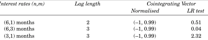
Table 3: Johansen Procedure on Rt(n) and r t(m)
Interest rates (n,m) Lag length Cointegrating Vector
Normalised LR test
(6,1) months 2 (–1, 0.99) 0.51
(6,3) months 3 (–1, 0.99) 0.04
(3,1) months 3 (–1, 0.99) 2.32
Notes: In the Johansen procedure both the maximum eigenvalue test and the trace test
do not reject the null of a unique co-integrating vector. The likelihood ratio (LR) statistic in column 4 tests the null that the co-integrating vector is (–1,1). Under the null, the reported test statistic has a critical value (at 5 per cent significance level) of 3.84.
4.3 The Spread and the Predictability of Changes in Short Rates
[image:9.499.68.426.138.207.2]The regression of the perfect foresight spread, PFSt(n,m) on the actual spread St(n,m) and the limited information set Ht (consisting of lags of St(n,m) and ∆rt(m)) are shown in Table 4. In all cases we do not reject the null of H0:β=1 or that information, available at time t or earlier does not incrementally add to the predictions of future interest rates. We also do not reject the null that the constant term premium is zero (i.e. α = 0). The results therefore do not reject the EH + RE.
Table 4: Does the Spread Predict Future Changes in Short-Rates?
Regression: PFSt(n,m)= α + βS
t(n,m) + γ Ht
Spread (n,m) Coefficients Wald Test
α β H0:β=1 H1:α=0, H2:γ=0
s.e.(α) s.e.(β) β=1
[p-value] [p-value] [p-value]
(6,1) -0.001 1.04 0.09 0.08 0.32
(0.001) (0.15) [0.77] [0.78] [0.58]
(6,3) –0.0006 1.02 0.007 0.007 2.88
(0.0008) (0.32) [0.93] [0.93] [0.09]
(3,1) –0.001 0.87 0.38 0.39 3.75
(0.001) (0.21) [0.54] [0.53] [0.06]
Notes: The regression coefficients reported in columns 2 and 3 are from the regression
with γ = 0 imposed. The method of estimation is GMM with a correction for
hetero-scedasticity and moving average errors using the Newey-West (1987) declining weights. The last 3 columns report Wald statistics and marginal significance levels
for the null hypothesis stated. For H0:γ = 0 the reported results are for an
information set which includes 4 lags of the change in the interest rates and the
interest rate spread. The null H0:β=1, is conditional on γ=0 while the null H1:α=0,
β=1 is also conditional on γ=0.
4.4 The Theoretical Spread and the VAR Results
Table 5 contains the results from the VAR models for St(n,m) and ∆r
[image:10.499.72.430.216.285.2]t(m). The lag length is chosen to minimise the Akaike Information Criterion (AIC), except for the rare occasions when additional lags are required to avoid any serial correlation in the residuals. A weak test of the EH is that the spread Granger-causes changes in short-term interest rates and this is not rejected for all maturities (Table 5, column 3). There is also Granger-causality from ∆rt(m) to St(n,m) for the (6m,3m) case, indicating feedback in the VAR regression.
Table 5: VAR Model for (St(n,m), ∆r t
(m))
Spread Lag Granger Tests Causality Ljung- Box Q(26) R2- Statistic
(n,m) St on ∆rt(m) ∆rt(m) on St St– eqn. ∆rt– eqn St– eqn. ∆rt– eqn
(6,1) 2 <0.01 0.48 9.36 17.4 0.52 0.22
(6,3) 2 <0.01 <0.01 13.3 27.7 0.62 0.19
(3,1) 2 <0.01 0.50 11.3 18.8 0.38 0.26
Notes: “Lag” denotes the lag length that minimises the Akaike Information Criterion (AIC).
Where the latter (occasionally) results in an equation system with serial correlation, the AIC is overridden and extra lags added (back) until any residual serial correlation is eliminated. The critical value for Q(26) is 38.89 (5 per cent significance level). In columns 3 and 4 we report the marginal significance levels for the Granger-causality tests of St(n,m) on ∆rt(m) and vice versa (statistics are calculated after applying the GMM correction for heteroscedasticity used in Campbell and Shiller (1991)). The final 2 columns give the R2–statistic for each equation. The regressions are estimated for the whole sample period, January 1984 to October 1997.
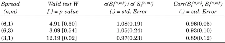
For illustrative purposes the graph of the actual spread St and the theoretical spread St’ are shown for (n,m) = (6, 1) and they move closely together, Figure 2. In the regression of St on St’ (Table 6) the point estimate of the slope coefficients are very close to unity, for all 3 maturity combinations. The intercepts in these regressions are not statistically significantly different from zero in each case. Table 7 provides the metrics for the relationship between the actual spread St and the theoretical spread St’. The results indicate that the VAR restrictions are not rejected. For all maturities there is a strong correlation (column 4) between the actual spread St(n,m) and the predicted (theoretical) spread St(n,m)’. The standard deviation ratio, SDR = σ(St(n,m)’)/ σ(St(n,m)) yields estimates (column 3) which are all within two standard errors of unity. The Wald test of the VAR cross equation parameter restrictions (Table 7, column 2), are not rejected for the (6m,3m) and (6m,1m) case, but are rejected for (3m,1m).
Table 6: Regression of the Actual Spread St on the Theoretical Spread St’
Interest Rate α β R2
Maturity statistic
coeff. s.e. coeff. s.e.
(6,1) –0.01 0.02 0.90 0.06 0.93
(6,3) 0.02 0.01 0.81* 0.07 0.87
(3,1) 0.02 0.03 0.83 0.13 0.80
Notes: The regressions are estimated for the whole sample period, January 1984 to
October 1997. The estimated regression is St = α + βSt’ + εt which is estimated by
GMM with heteroscedastic corrected errors. A star indicates the estimated coefficient is statistically different from that implied by the null hypothesis (at a
5 per cent significance level), which for ‘α’ is H0: α = 0 and for ‘β’ is H0: β = 1. The
theoretical spread St’ is obtained from the predictions from the VAR using z = [St,
∆rt].
the current spread St(n,m) on future changes in interest rates via the chain rule of
forecasting is less than required by the EH. However in contrast to (1) our single equation perfect foresight regressions in Table 4 reject the null that Ht influences future changes in interest rates. Hence rejection of the VAR restrictions is probably due to the “low weight” given to St(n,m) in the VAR regression. This may
occur because over short forecasting horizons one might expect agents to utilise almost minute by minute observations of St(n,m) and ∆R
t
(m) and hence forecasts
based on monthly data might not adequately mimic such behaviour for the (3m,1m) maturities.
Figure 2: Actual and Theoretical Spread (6m - 1m)
-8 -7 -6 -5 -4 -3 -2 -1 0 1 2
198403 198409 198503 198509 198603 198609 198703 198709 198803 198809 198903 198909 199003 199009 199103 199109 199203 199209 199303 199309 199403 199409 199503 199509 199603 199609 199703 199709
actual theoretical
[image:11.499.67.427.325.407.2]Table 7: Tests of the EH Using Weakly Rational Expectations
Spread Wald test W σ(St(n,m)′)/σ( St(n,m)) Corr(St(n,m), St(n,m)′)
(n,m) [.] = p-value (.) = std. Error (.) = std. Error
(6,1) 4.91 [0.30] 1.08(0.19) 0.96(0.05)
(6,3) 3.09 [0.54] 1.05(0.24) 0.93(0.10)
(3,1) 12.19 [0.02] 0.97(0.23) 0.89(0.12)
Notes The regressions are estimated for the whole sample period, January 1984 to
October 1997.
V INTERPRETATION OF RESULTS
In this section we analyse our results and compare them with those from other studies. On balance our results favour the EH. The perfect foresight regressions (Table 4), the standard deviation ratios σ(St(n,m)’)/ σ(St(n,m)), and the coefficient of determination Corr(St(n,m), S
t(n,m)’) (Table 5), are consistent with the EH and this may be contrasted with the rejection of the VAR cross-equation restrictions for (3m,1m) combination in Table 5.10
First, the perfect foresight spread regressions implicitly allow potential future events (known to agents but not to the econometrician) to influence expectations, whereas the VAR approach requires the explicit information set known both to agents and the econometrician. Hence, if the econometrician erroneously excludes variables affecting traders’ perceptions, then the estimated VAR coefficients may be biased, resulting in rejection of the VAR cross equation restrictions. Second, if agents actually do use the VAR methodology for forecasting, one would expect them to utilise almost minute by minute observations of (St(n,m), ∆r
t(m)) : hence forecasts based on monthly data seem unlikely to adequately mimic such behaviour. Third, Campbell and Shiller (1991) have argued that rejection of the cross-equation parameter restrictions although statistically significant may not constitute a major departure form the EH on economic grounds, as long as the theoretical spread closely tracks the actual spread.11 Finally, the Monte Carlo evidence in Bekaert et al. (1997) and Bekaert and Hodrick (2000) shows that the Wald test suffers from severe size distortions and use of asymptotic critical values “results in gross over-rejection of the null”.
Our perfect foresight spread results are broadly consistent with the results in Cuthbertson (1996a); who found slope coefficients ranging from 0.73 to 1.3.
The author could not reject the null, H0:β=1, γ=0 which is consistent with the EH for the UK at the short end of the maturity spectrum. This is also consistent with Hurn et al. (1996) and Cuthbertson et al. (1996).12
Campbell and Shiller (1992) use monthly data on US government bonds for the period 1946 to 1986, and their results are broadly consistent with our reported results for the perfect foresight spread equations. However Campbell and Shiller find that the Corr(St(n,m), St(n,m)’) are relatively low being in the range 0-0.7 and the values of the variance ratio are in the range 2-10 for maturities of less than 1 year. Campbell and Shiller do not directly test the VAR cross-equation restrictions but this has been done subsequently by Shea (1992) who in general finds they are rejected. Again our results are generally consistent with those of Cuthbertson (1996a) using UK data at short maturities. Cuthbertson’s results from the VAR models for St(n,m) and ∆rt(m) indicate that St(n,m) Granger causes St(n,m) and ∆rt(m): a weak test of the EH.13 The author also finds that for all maturities there are strong correlations between the actual and theoretical spread, and that the variance ratios are close to unity. Hurn et al. (1996) using monthly LIBOR rates (1975-1991) find the VAR cross-equation restrictions are not rejected, while Cuthbertson (1996a) rejects these. Our results on Irish data are more informative than those of Hurley (1990), because of our longer and more accurate data set and the wider array of tests used. We find much more support for the EH than does Hurley (1990).
VI CONCLUSIONS
Using a number of short-term maturities on monthly Irish money market rates from 1982 to 1997, we perform a number of tests of the EH of the term structure of interest rates for Ireland. On balance our results would appear to lend support to the EH. Using the Johansen procedure on the 1-month, 3-month and 6-month interest rates we find that the cointegrating vector between any pair of interest rates is {1, –1} — this provides a “weak” test in favour of the EH. A regression of the future change in short rates (i.e. the perfect foresight spread) on the actual spread gives a coefficient of unity on the latter variable, which is again consistent with the EH. Turning to the bivariate VAR we find that the forecast of future changes in short rates (i.e. the theoretical spread) moves closely with the actual spread. Both the standard deviations ratio and the correlation
12. Campbell and Shiller (1991) use monthly US data from January 1952 to February 1987, and find little support for the EH at the short end of the maturity spectrum. The authors obtained slope coefficients β ranging between 0 and 0.5.They do find beta coefficients of around 1 for maturities of 4,5 and 10 years.
coefficients for the theoretical spread relative to the actual spread give results in favour of the EH. However, the VAR cross-equation restrictions although favourable to the EH for the (6,3) and (6,1) interest rate combinations, are not so for the (3,1) combination. However, we do provide a number of reasons why the cross-equation restrictions may be rejected (including the small sample evidence in Bekaert et al. (1997) and Bekaert and Hodrick (2000)), even though the EH remains a good representation of the data. It is encouraging that our results are consistent with recent studies which also focus on the short end of the maturity spectrum (e.g. Cuthbertson (1996a) for the UK and Engsted (1994) for Denmark).
REFERENCES
BEKAERT, G., and R.J. HODRICK, 2000. ‘Expectations Hypothesis Tests”, National Bureau of Economic Research Working Paper 7609, March.
BEKAERT, G., R.J. HODRICK, and D. MARSHALL, 1997. “On Biases in Tests of the Expectations Hypothesis of the Term Structure of Interest Rates”, Journal of Financial
Economics, Vol. 44, pp. 309-348.
BREEN, R., 1991. “Comment on Joyce (1991)”, Journal of Statistical and Social Inquiry
Society of Ireland, Vol. XXVI, Part iii, pp. 186-190.
BREEN, R. and G. KEOGH, 1990. “Modelling the Term Structure of Irish Interest Rates”, Paper delivered at UCC, 12 January 1990, Mimeo.
CAMPBELL, J.Y., and R.J. SHILLER, 1987). “Cointegration and Tests of Present Value Models”, Journal of Political Economy, Vol. 95, pp. 1062-1088.
CAMPBELL, J.Y., and R.J. SHILLER, 1991. “Yield Spreads and Interest Rate Movements: a Birds Eye View”, Review of Economic Studies, Vol. 58, pp. 495-514.
CUTHBERTSON, K., 1996a. “The Expectations Hypothesis of the Term Structure: The UK Interbank Market”, The Economic Journal, Vol. 106, No.436, pp. 578-592. CUTHBERTSON, K., 1996b. Quantitative Financial Economics, J. Wiley.
CUTHBERTSON, K., S. HAYES, and D. NITZSCHE, 1996. “The Behaviour of Certificates of Deposits Rates in the UK’, Oxford Economic Papers, Vol. 48, pp. 397-414.
ENGSTED, T., 1994. “The Predictive of the Money Market Term Structure”, Aarhus School of Business, Denmark (mimeo).
ENGSTED, T., and C. TANGGAARD, 1994. “A Cointegration Analysis of Danish Zero-Coupon Bond Yields”, Applied Financial Economics, Vol. 24, pp. 265-278.
EVANS, M.D.D., and K.K. LEWIS, 1994. “Do Stationary Risk Premia Explain it all?”
Journal of Monetary Economics, Vol. 33, pp. 285-318.
HALL, S.G., 1986. “An Application of the Granger and Engle Two-Step Estimation Procedure to UK Aggregate Wage Data”, Oxford Bulletin of Economics and Statistics, Vol. 48, No. 3, pp. 229-239.
HANNAN, E.J., 1970. Multiple Time Series, New York: Wiley.
HANSEN, L.P., 1982. “Large Sample Properties of Generalised Method of Moments Estimators”, Econometrica, Vol. 12, pp. 1029-1052.
HARDOUVELIS, G.A., 1994. “The Term Structure Spread and Future Changes in Long and Short-Rates in the G7 Countries”, Journal of Monetary Economics, Vol. 33, pp. 255-283.
Irish Case”, The Economic and Social Review, Vol. 22, No. 1, pp. 25-34.
HURN, A.S., T. MOODY, and V.A. MUSCATELLI, 1996. “The Term Structure of Interest Rates in the London Interbank Market”, Oxford Economic Papers, Vol. 47, No. 3, pp. 418-436.
JOHANSEN, S, 1988. “Statistical Analysis of Cointegrating Vectors”, Journal of Economic
Dynamics and Control, Vol. 12, pp. 231-254.
JOYCE, A., 1991. “The Development of Yield Curves for the Irish Securities Market”,
Journal of Statistical and Social Inquiry Society of Ireland, Vol. XXVI, Part III,
pp.109-185.
KUGLER, P., 1988. “An Empirical Note on the Term Structure and Interest Rate Stabilization Policies”, Quarterly Journal of Economics, Vol. 103, No. 4, pp. 789-792. MacDONALD, R., and A.E.H. SPEIGHT, 1991. “The Term Structure of Interest Rates Under Rational Expectations: Some International Evidence”, Applied Financial
Economics, Vol. 1 pp. 221-221.
MacKINNON, J.G., 1991. “Critical Values for Cointegration Tests”, in R.F. Engle and C.W.J. Granger (eds.), Ch. 13, Long-run Economic Relationships: Readings in
Cointegration, Oxford: Oxford University Press, pp. 267-276.
MANKIW, N.G., and J.A. MIRON, 1986. “The Changing Behaviour of the Term Structure of Interest Rates”, Quarterly Journal of Economics, Vol. 101, pp. 221-228.
McCULLOCH, J.H., 1971. “Measuring the Term Structure of Interest Rates”, Journal of
Business, Vol. 44, pp. 19-31.
McCULLOCH, J.H., 1975. “The Tax Adjusted Yield Curve”, Journal of Finance, Vol. 30, pp. 811-830.
McCULLOCH, J.H., 1987. “US Government Term Structure Data”, Department of Economics, Ohio State University (mimeo).
McGETTIGAN, D., 1995. “The Term Structure of Interest Rates in Ireland: Description and Measurement”, Central Bank Technical Paper 1/RT/95.
MELINO, A., 1988. “The Term Structure of Interest Rates: Evidence and Theory”, Journal
of Economic Studies, Vol. 2, No. 4, pp. 335-366.
NEWEY, W.K., and K.D. WEST, 1987. ‘”A Simple Positive Definite Heteroscedasticity and Autocorrelation Consistent Covariance Matrix”, Econometrica, Vol. 55, pp. 703-708. PHILLIPS, P.C.B., and P. PERRON, 1988. “Testing for a Unit Root in Time Series
Regression”, Biometrica, Vol. 75, No. 2, June, pp. 335-346.
RUDEBUSCH, G.D., 1995. “Federal-Reserve Interest-Rate Targeting, Rational Expectations, and the Term Structure”, Journal of Monetary Economics, Vol. 35, No. 2, pp. 245-274.
SHEA, G.S., 1984. “Pitfalls in Smoothing Interest Rate Term Structure Data: Equilibrium Models of the Term and Spline Approximations”, Journal of Financial and Quantitative
Analysis, Vol. 19, pp. 253-269.
SHEA, G.S. (1992) “Benchmarking the Expectations Hypothesis of the Term Structure: An Analysis of Cointegration Vectors”, Journal of Business and Economics Statistics, July, pp. 347-365.
SHILLER, R.J., 1989. Market Volatility, Cambridge, Massachusetts: MIT Press. TAYLOR, M.P., 1992. “Modelling the Yield Curve”, The Economic Journal, Vol. 102, No.
412, pp. 524-537.