UW Biostatistics Working Paper Series
12-19-2003
Semiparametric Estimation of Time-Dependent:
ROC Curves for Longitudinal Marker Data
Yingye Zheng
Fred Hutchinson Cancer Research Center, [email protected]
Patrick Heagerty
University of Washington, [email protected]
This working paper is hosted by The Berkeley Electronic Press (bepress) and may not be commercially reproduced without the permission of the copyright holder.
Copyright © 2011 by the authors
Suggested Citation
Zheng, Yingye and Heagerty, Patrick, "Semiparametric Estimation of Time-Dependent: ROC Curves for Longitudinal Marker Data" (December 2003).UW Biostatistics Working Paper Series.Working Paper 220.
1. Introduction
Recent developments in molecular technology such as gene-expression microarrays and proteomics have led to a surge in research aimed at discovering markers useful for disease screening or for providing patient prognosis. We consider a marker to be any measurement that has the potential to signal the onset or progression of disease. Examples of potential markers include prostate specific antigen (PSA) as an indicator of prostate cancer, or pulmonary function measures such as forced expiratory volume (FEV1) as an indicator of functional decline prior to death among cystic fibrosis patients. Longitudinal marker analysis seeks to evaluate whether changes in a marker process correlate with a key clinical event time such as disease onset or death. Ideally a marker process would provide definitive and early information regarding disease onset. However, in practice most biological measurements contain substantial variability which complicates their use in guiding health care decisions. Characterizing the accuracy of time-varying markers for disease detection is therefore a critical step in the marker discovery process.
Retrospective longitudinal studies can be useful in a key phase of marker development (Pepe, Etzioni, Feng, Potter, Thompson, Thornquist, Winget and Yasui 2001). With this design the ca-pacity of a marker to detect preclinical disease can be evaluated as a function of time prior to the clinical occurrence of signs and symptoms. The scientific goal is to identify markers that exhibit high discriminatory ability at relatively early stages of disease. Traditionally in medical diagnostic research the receiver operating characteristic (ROC) curve is used to summarize the accuracy or dis-crimination potential of a marker measurement. (Hanley 1989; Zweig and Campbell 1993). However, to characterize early disease detection the cross-sectional concepts of sensitivity and specificity that are typically displayed in an ROC curve need to be extended to incorporate both the time-varying nature of a marker and the clinical onset time of the disease. In this article we consider new semipara-metric statistical methods for estimating time-dependent sensitivity, specificity, and ROC curves that adopt weak distributional assumptions. In addition, we develop the asymptotic distribution theory that allows inference for either time-dependent sensitivity and specificity, or for time-dependent ROC curves. Our methods also allow accuracy summaries to depend on covariates, and thus can be used to evaluate whether the accuracy of a marker varies across patient subgroups.
In the classic diagnostic testing setting, disease status is represented by a binary variable Di
for subject i. Furthermore, the relationship between Di and a continuous test result Yi for a given
subgroup defined by a covariate vectorZiis displayed through a conditional ROC curve. A conditional
ROC curve displays the full spectrum of values for sensitivity, or the “true positive rate” (TP),P(Yi<
c|Di = 1,Zi), and 1 minus the specificity, or the “false positive rate” (FP), 1−P(Yi ≥c|Di = 0,Zi)
by considering all possible test threshold valuesc. Therefore, an ROC curve is a plot of TP versus FP
forc∈(−∞,∞). In our definitions for TP and FP we assume that a low marker value is indicative of
disease, but parallel definitions can be adopted when high marker values are associated with disease. When tests are measured longitudinally, we can define TP and FP as time-dependent functions
T P(s, c|t,Zi) = P[Yi(s)< c|Di(t) = 1;Ti > s,Zi] (1.1)
F P(s, c|t,Zi) = P[Yi(s)< c|Di(t) = 0;Ti > s,Zi]. (1.2)
Here Yi(s) indicates a marker measured at time s, with s ≥ t0, the baseline time, and Di(t) is a
binary variable indicating the disease status of subject iat time t. We recognize that there can be
two useful time-varying “case” definitions to obtain Di(t) = 1 based on the disease timeTi: if we are
interested in the incidence of the disease at time t, then we can defineDi(t) = 1 when Ti =t; if we
are interested in the prevalence of the disease by time t, we can defineDi(t) = 1 whenTi ≤t.
In this manuscript we focus on incident ROC curves defined as a plot of [T PI
(s, c|t,Z), F PC
(s, c|t?,Z)]
for all possiblec, where
T PI(s, c|t,Zi) = P[Yi(s)< c|Ti =t;Zi, Ti > s] (1.3)
F PC(s, c|t?,Zi) = P[Yi(s)< c|Ti > t?;Zi, Ti> s] . (1.4)
Here, we uset? in the definition ofF P to denote as controls those subjects that do not experience the
disease prior to a fixed follow-up time. This definition is useful when some subjects are thought to
avoid disease and may reasonably be identified as the “long term survivors” characterized byTi> t?.
Incident ROC curves are most useful in a retrospective study when the timing of diagnosis for diseased patients is certain.
Incorporating the time dimension in ROC analysis has recently been discussed by a number of authors (Etzioni et al. 1999; Slate and Turnbull 2000; Heagerty, Lumley and Pepe 2000; Cai and Pepe 2002). Non-parametric methods that characterize accuracy using disease prevalence for the
case definition, Di(t) = 1(Ti ≤ t), is given in Heagerty et al. (2000). Other authors have used
the incident case definition, Di(t) = 1(Ti = t), including Etzioni et al. (1999), Slate and Turnbull
(2000), and Cai and Pepe (2002). There are two general approaches to characterizing accuracy and to calculating covariate specific ROC curves. First, direct regression approaches for ROC analysis have been proposed (see Pepe (1998) and Pepe (2003) for reviews). These methods use generalized linear model concepts to characterize the shape of the ROC curve and to allow covariates to directly impact accuracy. For longitudinal data Etzioni et al. (1999) illustrate the ROC-GLM approach for evaluating time-dependent accuracy. Despite recent work that permits flexibility in the direct ROC regression approach (Cai and Pepe 2002; Li, Tiwari and Wells 1999), the methods have not been extended to allow covariates to impact the link function, and thus potentially place restrictions on how the shape of the ROC curve varies with covariates. The semi-parametric methods that we introduce in section 2 permit the shape of the ROC curve to change smoothly with covariates.
A second general approach to estimating covariate specific ROC curves is based on modelling of the marker distribution conditional on disease status and covariates. Given estimates of the marker distribution for cases and controls an induced covariate specific ROC can be calculated (Tosteson and Begg 1988). For longitudinal markers Etzioni et al. (1999) and Slate and Turnbull (2000) discuss a parametric regression approach that uses linear mixed models to characterize the longitudinal marker
distribution for diseased and non-diseased subjects. In this approach the disease onset time, Ti, is
an additional covariate for the cases only. Our proposal is to use smooth semi-parametric regression quantile methods to model the marker distribution as a function of disease status, covariates, and disease onset time for the cases. By using flexible regression quantile methods we can relax the distributional assumptions adopted by previous proposals.
In section 2 we describe the estimation and inference procedures. We outline the asymptotic distribution theory for the proposed estimators in section 3. We use pulmonary function data from cystic fibrosis patients to illustrate the method and to compare semi-parametric analysis results to
parametric results.
2. Semiparametric Regression Quantile Method
2.1 Notation
In many studies subjects are classified either as disease cases or as controls on the basis of the
observed event time. For example, control subjects may be defined as individuals who after t? time
units remain free of disease, while cases are individuals with an observed event time,Ti < t?. Here we
consider a case-control study setting, where there arenD cases andnD¯ controls amongnsubjects (i.e.,
n =nD +nD¯). Let Yik be the continuous random variable representing the marker value obtained
from the ith case at the kth visit time sik, with i = 1, . . . , nD, and k = 1, . . . , Ki. For cases let
ZTik =vec(Ti, sik,Xi), orZD, denote a vector of covariates associated withYik, where Xi denotes a
vector of covariates that do not change with time. The total number of observations from the case
population isND =Pin=1D Ki. Similarly, denoteYjlas the marker value obtained from thejth control
at the lth visit time sjl, with j = nD + 1, . . . , nD +nD¯, and l = 1, . . . , Lj. For controls let Zjl or
ZD¯ denote a vector of covariates associated with Yjl. Since there are no disease diagnosis times for
controls,ZTjl=vec(sjl,Xj) withXj as the time-independent covariate vector for thejth control. The
total number of observations for the control group is ND¯ =Pnj=1D¯ Lj. We thus have N =ND +ND¯
observations from the two populations.
2.2 Semiparametric Estimation of Regression Quantiles
We propose to use semiparametric regression quantile estimation in order to construct time-dependent ROC curves. Similar to the methods of Heagerty and Pepe (1999), we characterize the conditional
distribution of [Yik|Zik] as from a location-scale family. Specifically, we represent a case marker value
as
Yik =µD(Zik) +σD(Zik)D(Zik) (2.1)
whereµD and σD are the location and scale functions, and the baseline distribution function for D
is
We characterize the conditional distribution of the marker measured from the control population
in the same way, withµD¯ andσD¯ representing the location and scale functions, and with the baseline
distribution function denoted
G0,zD¯() =P[D¯(Zjl)≤|Zjl]. (2.3)
As in Heagerty and Pepe (1999), for continuous ZD, we model µD(Zik) and σD(Zik) as smooth
functions ofZparametrically using regression splines:
µD(Zik) = P X p=1 βpRp(Zik) (2.4) logσD(Zik) = Q X q=1 γqSq(Zik) ; (2.5)
where Rp(Zik) and Sq(Zik) are regression spline basis functions. Heagerty and Pepe (1999) used
a quasi-likelihood method for estimation. For example, to estimate ˆβp and ˆγp (for p = 1, . . . , P)
associated with the case population, we can simultaneously solve the following estimating equations:
nD X i=1 Ki X k=1 R(Zik)T[Yik−µD(Zik)]/σ2D(Zik) = 0 (2.6) nD X i=1 Ki X k=1 S(Zik)T{[Yik−µD(Zik)]2−σ2D(Zik)}/σD2(Zik) = 0 (2.7)
Estimation for µD¯ and σD¯ follows in a parallel fashion.
Similar to Heagerty and Pepe (1999), the baseline distribution functions F0 and G0 are left
unspecified, and can be estimated empirically based on the standardized residual ikD =D(Zik) =
[Yik−µD(Zik)]/σD(Zik) and jlD¯ = D¯(Zjl) = [Yjl−µD¯(Zjl)]/σD¯(Zjl). If the distributions of the
standardized residuals are independent of covariates, the natural estimators for F0 and G0 are the
empirical distribution functions of the forms ˆ F0() = nD X i=1 Ki X k=1 1 ND 1(ˆikD ≤) (2.8) and ˆ G0() = n¯ D X j=1 Lj X l=1 1 ND¯1(ˆjlD¯ ≤), (2.9)
where ˆikD = [Yik −µˆD(Zik)]/σˆD(Zik) and ˆjlD¯ = [Yjl−µˆD¯(Zjl)]/σˆD¯(Zjl). However, more general
In this manuscript we consider the symmetrized nearest neighbor (SNN) estimator (Yang 1981) for the conditional baseline distribution function, which is defined as a weighted sum
ˆ F0(|Z, an) = nD X i Ki X k 1 W(Z)wan(Z,Zik)1(ˆikD ≤) (2.10)
where W(Z) = Pwan(Z,Zik) and an is a bandwidth parameter. A general form for wan can be
assumed with wan(Z,Zik) =K Hn(Z)−Hn(Zik) an (2.11)
where K(·) is a continuous and bounded probability kernel on [-1,+1], Hn(·) is the empirical
distri-bution function of Z. An SNN estimator for G0(|Z, an) can be similarly defined. In the following,
we use the notation F0,zD, G0,zD¯ and F0(|Z=zD, an),G0(|Z=zD¯, an) interchangeably.
2.3 Semiparametric Regression-Quantile-Based Estimator of ROC Curves
We now construct an estimator for a time-dependent ROC curve based on the semiparametric
regres-sion quantile estimators. We estimate an ROC curve for a given covariate value Zby first modeling
the marker as functions of covariates ZD for the cases or ZD¯ for controls. By using the
semipara-metric regression quantile methods to model the marker, we can derive a semiparasemipara-metric estimator for conditional ROC curves. For convenience, we define a positive test as a marker value less than a certain threshold, and thus the true positive rate (TP) is defined in terms of the cumulative
distri-bution function F(c) instead of survival function 1−F(c). For any false positive ratep∈[0,1], our
proposed estimator for the ROC curve is
\ ROCz(p) = Fˆ0,zD ˆ µD¯(zD¯)−µˆD(zD) ˆ σD(zD) + ˆG−0,1zD¯(p) ˆ σD¯(zD¯) ˆ σD(zD) ≡ Fˆ0,zD h ˆ α0+ ˆG−0,1zD¯(p)ˆα1 i (2.12) where F0,zD, G0,zD¯, µD(zD), µD¯(zD¯), σD(zD) andσD¯(zD¯) are defined as in section 2.2. ˆG−
1
0,z¯
D(p) is
the conditional empirical quantile function, with ˆG−0,1z¯
D(p) =inf[: ˆG0,zD¯()≥p].
3. Asymptotic Distribution Theory for ROC Curve Estimators
In this section we derive the large sample properties of our semiparametric ROC estimators. We first consider an ROC curve estimator that assumes the baseline distribution functions do not vary with
covariates Z. We then consider an ROC curve estimator based on SNN estimation of the baseline distribution function, assuming dependence on covariates. Proofs for the main theorems are detailed in the appendix.
Hsieh and Turnbull (1996) studied the asymptotic properties of a nonparametric ROC estimator
of the formF[G−1(p)], and a semiparametric ROC estimator where the distributions of F andGare
normal. In the simplest situation where there are no covariates and each subject contributes a single observation, our estimators reduce to that of Hsieh and Turnbull (1996).
3.1 Baseline Distribution Functions Are Independent of Covariates
When baseline functions are independent of covariates, we use equation 2.8 and equation 2.9 to
estimate the baseline distribution functions F0 and G0.
For asymptotic results we assume the following regularity conditions:
• F0, G0 are continuous with continuous densities f0, g0, respectively.
• The slope of the ROC curve f0[α0+G−01(p)α1]/g0[G−01(p)], is bounded on any interval (a, b),
with 0< a < b <1.
• nD/n→λ >0 as n→ ∞.
• The number of observations per subject is relatively small with respect to n, the total number
of subjects. i.e., we assumeND/nD →cD andND¯/nD¯ →cD¯.
Theorem 1 (Consistency of ROC curve estimator) Under the conditions above,
sup
0≤p≤1|
\
ROCz(p)−ROCz(p)| →0 a.s. as n→ ∞.
Theorem 2 (Asymptotic normality) Under the conditions above, there exists a probability space on which one can define sequences of two independent zero-mean Gaussian variables[U1(p), U2(p),0≤
p≤1 ] respectively such that for 0< a < b <1,
√
n[\ROCz(p)−ROCz(p)]→Ψ(p),a.s. as n→ ∞ uniformly on [a,b]. with Ψ(p) = 1 cD √ λU1(p) + 1 cD¯√1−λ α1 f0[α0+G−01(p)α1] g0[G−01(p)] U2(p)
We specify the forms forU1(p) andU2(p) in the appendix.
3.2 Baseline Distribution Functions Are Smooth Functions of Covariates
In this section we provide asymptotic results for the situation in which baseline functions are smooth
functions of covariates. We use equation (2.10) to estimate the baseline distribution functions F0,z
and use a similar procedure forG0,z.
In addition to the assumptions in section 3.1, we also require the following:
• K(x) is twice continuously differentiable probability kernel which vanishes outside some finite
interval.
• (an)n is a sequence of bandwidths converging to zero, andna3n→ ∞ asn→ ∞.
• Zhas continuous distribution function H(·).
Theorem 3 (Consistency) Under the conditions above,
sup
0≤p≤1|
\
ROCz(p)−ROCz(p)| →0 a.s. as n→ ∞.
Theorem 4 (Asymptotic normality of SSN ROC estimator) Under the conditions above, there exist a probability space on which one can define sequences of two independent zero-mean Gaussian random variables [U1?(p), U2?(p), 0≤p≤1 ] such that for 0< a < b <1,
√
nan[\ROCz(p)−ROCz(p)]→Ψ(p),a.s. as n→ ∞ uniformly on [a,b]. with Ψ(p) = 1 cD √ λU ? 1(p) + 1 cD¯√1−λ α1 f0,z[α0+G−0,1z(p)α1] g0,z[G−0,1z(p)] U2?(p)
We specify the forms forU1?(p) and U2?(p) in the appendix.
3.3 Bandwidth Selection
Methods that guide the selection of smoothing parameters facilitate optimal estimation by balancing bias and variance. In practice one can either employ cross-validation to select a bandwidth that minimizes a pre-specified loss function, or adopt a data-driven procedure to estimate the asymptot-ically optimal bandwidth. Ideally if the statistical objective is to estimate conditional ROC curves
then a criterion focusing directly on key aspects of the ROC curve would be desirable. However, our methodology is “indirect” in that we first model the marker distribution separately for cases and controls, and then construct the induced conditional ROC curves. Given our approach, we adopt an optimal bandwidth selection strategy that is based on the asymptotic distribution of conditional quantile estimators for the cases and the controls.
For either cases or controls a given percentile p ∈ [0,1] defines a quantile function p(x) =
F−1(p|x). A theoretical bandwidth that minimizes the asymptotic integrated mean square error
(IMSE) is of the forman= (b/n)1/5, with
bopt(p) = Z σ2[ p(x)|x] {f[p(x)]|x}2 dx / µ2 Z ω[ p(x)|x] f[p(x)|x] 2 dx ! (3.1)
where σ2[p(x)|x] is the variance of the estimator of F[p(x)|x, an], ω[p(x)|x] denotes the second
derivative of the smoothed conditional empirical process evaluated at p(x), andf[p(x)|x, an] is the
conditional density function for ij evaluated at p(x). Ducharme, Gannoun, Guertin and J´equier
(1995) give a detailed discussion of estimation for the necessary components in equation (3.1) when
analyzing independent data. For dependent data we simply modify the estimate ofσ2[p(x)|x] using
a robust variance estimator (see the appendix for details). Since bopt involves unknown quantities
such asσ2[p(x)|x] and ω[p(x)|x], in applications we simply use a plug-in estimator by first choosing
an arbitrary a∗n of order n1/5, and then estimating the terms in bopt(p) based on the preliminary
estimates using a∗n.
Note thatbopt(p) is a function ofpand therefore may vary for different percentile values. In ROC
analysis we seek to estimate the entire distribution function (all quantiles) rather than focus on a single
percentile value,p. However, not all values for the false positive rate are scientifically important, and
in general interest primarily targets the true positive rate (sensitivity) that corresponds to low false
positive rates (1-specificity). Therefore, for controls we considerbopt(p) calculated for a range of values
such as 0.75< p <0.95, and for cases we consider a slightly wider range such as 0.60< p <0.95. For
cases and controls, we then evaluate the range of optimal bandwidths and for each group we choose a single value which is nearly optimal over the percentiles of interest. Further work is warranted toward developing an optimal bandwidth selection algorithm that is specially tailored for ROC analysis.
4. Example: Cystic Fibrosis Data 4.1 Study Description
The cystic fibrosis (CF) data we analyze come from the U.S. Cystic Fibrosis Foundation (CFF) National Patient Registry, a database of patients with CF seen at CFF-accredited care centers. The registry has been updated annually since 1966 and contains longitudinal measures of participant health status. Registry information available from 1990-1998 provides 9 years of follow-up on 21,138
patients for a total of N = 171,306 observations. During the follow-up period, 8.52% of the patients
died and thus most of the longitudinal marker information comes from patients who remain alive through the end of the observation period.
In the subsequent analysis we focus on a standardized pulmonary function measurement known as FEV1 percent-predicted. This outcome measures the volume of air that a subject expires in 1 second, and standardizes by dividing the raw volume by the age and gender specific population reference value. Thus, an FEV1 of 100 indicates that a subject has 100% of the expected lung function for a healthy child of his/her age. Currently, children are registered for lung transplantation if their FEV1 drops below a value of 30 (Davis 1997). One clinical question is whether this is an accurate decision threshold, and whether an age-specific criterion might be warranted. Specifically, what is the accuracy of the decision guideline? Does this identify most children who would otherwise die in the near future, and does it capture few of the children who are likely to survive? To examine the prognostic value of FEV1 at various ages we characterize age-specific sensitivity and specificity. By estimating conditional quantiles we can compute the threshold value that correctly identifies a given percent of children who do progress to death (i.e. the sensitivity), and similarly the threshold value that incorrectly identifies a given percent of children who do not progress to death (i.e. the false positive rate, or 1-specificity). Furthermore, by creating age-specific ROC curves we can determine whether controlling the false positive rate at a low value such as 10% leads to adequate sensitivity, and whether the threshold required to achieve good specificity suggests using a decision cut-off value that depends on age.
To address the scientific questions we conduct a case-control analysis. A case-control study for this application has several advantages. First, the sample size of the original CF data is considerable
and therefore a full cohort analysis would be computationally demanding. Second, the dataset is well suited for a case-control study since the outcome of interest, death, is rare and the exposure of interest is commonly available. Therefore, we should be able to estimate an effect comparable to that obtained from a full cohort analysis without much loss of statistical efficiency. Finally, as our analysis is essentially retrospective and only requires the measurement time (age) and the time of death we circumvent the issue of defining an appropriate time origin which would be required for proper prospective analysis.
In the CF sample we have 21,138 patients, of whom 1,496 died within the follow up period. For each of the observed cases, we assign two matched controls by selecting subjects who had been followed for more than 5 years and who are still alive at the end of the study. Furthermore, for the controls we exclude any observations that were obtained during the last five years before their final study visit so that all measurements included for analysis were taken at least 5 years before death. Thus the controls are defined here as those subjects who are ‘known’ to be healthy at the time FEV1 is measured; ‘known’ because death did not occur for at least 5 years. Controls are matched to cases by age at study entry. The resulting analysis data contain 1,496 cases and 2,992 control subjects with a total of 15,594 pulmonary function measurements.
The top panel of Figure 1 shows the association between FEV1 and subject age at measurement time. We use smoothed curves to describe FEV1 as function of age. As expected, the trends are for FEV1 to decrease with age for both cases and controls. This is consistent with the fact that decline of pulmonary function with increasing age is a recognized consequence of the disease process. The data suggest that the distribution of FEV1 is clearly different for cases as compared to controls, and this discrepancy may also vary with age. The association between FEV1 and time relative to death for the cases is displayed in the bottom panel of Figure 1. We see that FEV1 tends to be lower at times close to the time of death compared to times further from death.
In order to estimate ROC curves and to determine whether they vary with age and with time before death for cases, we fit a series of regression models. For comparison, models are fit both parametrically using the method described by Etzioni et al. (1999), and using a semi-parametric regression quantile method introduced in section 2.3. Although we focus on the current FEV1 value as the marker, other
derived outcome measures that are a scalar function of the current and/or past response process could
be candidate markers. For example, the change in FEV1,Y∗
ik(s) =Yik(s)−Yik(s−1), may represent a
marker that reflects failing pulmonary function. However, recent epidemiologic work suggests that the current level of FEV1 rather than change in FEV1 is predictive of death (Liou, Adler, FitzSimmons, Cahill, Hibbs and Marshall 2001). Below we briefly summarize the models for FEV1.
4.2 Parametric estimation of ROC curves
For the parametric approach, we use a linear mixed model for FEV1. For cases, we consider two
covariates for the kth measurement of subject i: age at which FEV1 is recorded (sik =ageik), and
years before death (Ti −sik =yearsBDik). Denote Zik = (sik, Ti−sik)T = (ageik, yearsBDik)T,
the model takes the form
E[F EV1ik|Zik, bi] =b0,i+b1,i·ageik+β0D+β1D·ageik+β2D ·yearsBDik+β3D·ageik·yearsBDik,
For the lth measurement of control subjectj, denote Zjl= (sjl) = (agejl). We assume
E[F EV1jl|Zjl, bj] =b0,j+b1,j·agejl+β ¯ D 0 +β ¯ D 1 ·agejl .
The models for both cases and controls assume a random intercept and a random slope for age.
Maximum likelihood estimates for the linear mixed models provide estimates for the means (µD,
and µD¯) and standard deviations (σD and σD¯). Assuming normality for both the case and control
populations leads to an induced ROC model:
ROCZ(p) = Φ µ ¯ D(ZD¯)−µD(ZD) σD(ZD) +σD¯(ZD¯) σD(ZD) Φ−1(p) ,
with Φ denotes the cumulative standard normal distribution. Table 1 summarizes the parameter estimates for the linear mixed models.
Figure 2 displays the induced ROC curves at various times before death for FEV1 measured at age 10, 15 and 20. At all ages, we see that the discrimination is better when FEV1 is measured at times closer to death. For example, at age 15, with a threshold of 39.17 for defining “test positive” (90% of
the controls are “test negative”), 60.3% of subjects who subsequently die at age 15 (the same year)
years prior to death), only 30.6% are “test positive”. Using this approach, there does not appear to be a trend in accuracy with age (Table 2). For example, if the false positive rate is controlled at 10% them when FEV1 is measured at the year of death (the time at which FEV1 is the most accurate), 57% of the children at age 10 are identified as “test positive”, whereas for FEV1 measured at age 20, 59% of those patients who died at age 20 were identified as “test positive”.
4.3 Semiparametric Regression Quantile Estimation of ROC curves
Separate models are now considered using the semiparametric regression quantile method to char-acterize the marker distributions for cases and controls. For controls, we model the mean function as µD¯(ZD¯) =β ¯ D 0 + (βββ ¯ D)TB(age)
and the logarithm of the standard deviation as
logσD¯(ZD¯) =γ0D¯ + (γ ¯
D)T
B(age)
whereB(age) is a natural spline basis with knots at 10 and 20 years. For the baseline distributionG0
we chose either to use ˆG0(D¯), the empirical distribution function of the standardized residuals, or
use the locally weighted empirical distribution function ˆG0(D¯|age, an), where we consider distance
based on age.
For cases, we model the mean function as
µD(ZD) =β0D+ (βββD)T[B(age)· B(yearBD)] and the logarithm of the standard deviation as
logσD(Z) =γ0D+ (γD)T[B(age) +B(yearBD)]
where B(age) is a natural spline basis with knots at 10 and 20, and B(yearBD) is a natural spline
basis with knots at 2 and 4 years. For baseline distribution F0 we chose either to use ˆF0(D), the
empirical distribution function of the standardized residuals, or use the locally weighted empirical
distribution function, where we consider distance based on either age only, ˆF0(D|age, an), or years
3
4(1−x2)I{|x| ≤1}and we select a bandwidth such that about 20% of the observations are included
for estimation at each unique value of Z. This bandwidth is selected based on a data-driven optimal
bandwidth selection algorithm described in section 3.3, and the estimated optimal bandwidths do
not appear to vary much when 0.75≤p≤0.95. For example, the bandwidth estimates for the cases
given by (3.1) arebbopt(0.75) = 0.134 andbbopt(0.95) = 0.143.
For controls, we observe a trend for the estimated mean FEV1 function ˆµD¯ to decrease with
increasing age. The standard deviation function, however, does not appear to vary much between 10 to
30 years of age. We also examine plots (not shown here) of the baseline distribution function ˆG0(|age),
and the estimated percentiles of FEV1 as function of age based on the semiparametric quasi-likelihood
method: ˆµD¯(age)+ˆσD¯(age) ˆG0(D¯|age). Both the baseline distribution and equivalently the estimated
percentiles appear to depend on age.
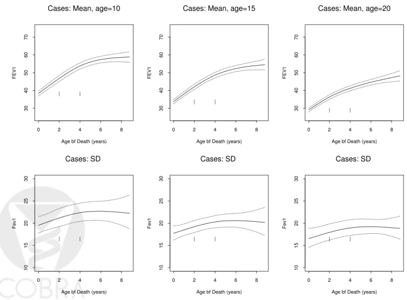
For cases, we examine the estimated mean ˆµD and the estimated standard deviation ˆσD as a
function of year before death for various ages (Figure 3). We see that the mean function at age 10 is generally higher than that at age 20, similar to the trend observed for controls. For each age, FEV1 level appears to increase as the time relative to death increases from 0 to four years, then gradually levels off. The standard deviation function follows a similar pattern, but to a lesser extent. We also
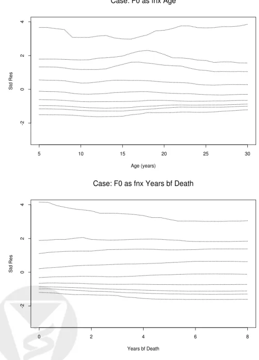
check plots (Figure 4) that show the baseline distribution function as a function of age, ˆF0{|age}, and
as a function of years before death, ˆF0{|yearBD}. For both situations, higher percentiles appear to
vary with covariates more than lower percentiles. This suggests that a variable baseline distribution estimator may be more appropriate than a constant baseline assumption for these data.
We compare the empirical distribution of the standardized residuals with a standard normal distribution, for cases, the empirical percentile is generally higher than the Gaussian percentile in the left part of the distribution (below 30%), but it tends to be lower than the Gaussian percentile between 30% and 90%. QQ-plot (not shown) also reveals right skewness. This implies that the normal assumption may not be plausible for these data. In contrast, for controls the empirical percentile is in good agreement with the Gaussian percentile, and the QQ-plot reveals little skewness.
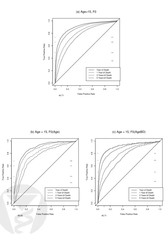
ROC curves at various times before death for 15 year olds are displayed in Figure 5. We compare
depends on age (panel (b)), and those that assumeF0 depends on the year before death (panel (c)). Similar to the findings with the parametric method, we observe better discrimination between cases and controls when FEV1 is measured at times closer to death across all ages and regardless of the
specific assumptions onF0. However, the ROC curves at 0, 1, 3, 5 years before death are considerably
different depending on the assumption about F0: the ROC curves at various times before death are
relatively closer to each other if we use the empirical distribution of the standardized residual to
estimate F0, in contrast to the ROC curves obtained by letting F0 vary with the time relative to
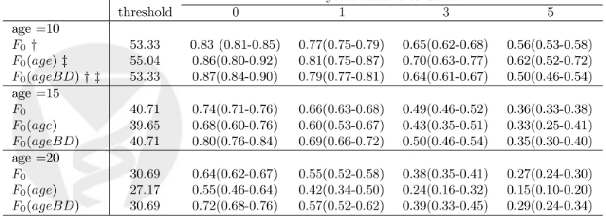
death. This can also be seen from Table 3, which lists the estimated sensitivities when specificity
equals 0.9. For example, at age 15, with an FEV1 value of 41 as the threshold for defining “test
positive”, 90% of the controls (those who lived at least beyond 20 years and are known to be alive
by the end of the study) are “test negative”. When F0 is assumed to be constant, the fraction of
subjects who are test positive are 74%, 66%, 49%, and 36% among those CF patients who die at age
15, 16, 18, and 20, respectively. However, if F0 depends on the time relative to death, then with the
same threshold, the corresponding true positive fractions become 80%, 69%, 50%, and 35%, which for 0 and 1 year prior to death are meaningfully different from the estimates obtained based on the other assumptions. Furthermore, comparing Table 3 with Table 2, we see there are also discrepancies between the estimates from the parametric method and those from the semi-parametric method. In order to estimate an ROC curve, we need to carefully characterize all components of the distribution, including the mean, the standard deviation, and the baseline distribution function. Misspecification of any of the three components may result in biased estimates of sensitivity and specificity.
The next logical step is to chose a model that best describes the baseline distribution. Developing a formal model selection procedure in the semi-parametric setting appears to be difficult. Instead, we suggest employing graphical summaries to assess whether the baseline distribution appears to vary with covariates. For example, we can utilize QQ-plots to compare the distribution of the standardized
residuals across different values of a covariate. In Figure 6, we plot the quantiles of residuals at k
years prior to death against the quantiles of residuals at k+ 1, . . . ,8 years prior to death for cases.
Many QQ-plots in the figure appear to be curved, indicating that the baseline distribution may not be constant over years prior to death. In contrast, when we examine the baseline distribution across
different ranges of age most of the QQ-plots are close to diagonal lines, and this is especially true for
controls. Thus, the assumption that G0 does not depend on age may be plausible for the data from
controls.
We also fit the same models using a Gaussian kernel function instead of the Epanechnikov’s kernel function to estimate the baseline distributions. The estimated sensitivities are similar to those in Table 3, indicating that the choice of the kernel function does not have substantial impact on the estimation.
5. Summary
In this article, we introduce an approach for constructing time-dependent ROC curves that is based on the semi-parametric regression quantile method for longitudinal data studied by Heagerty and Pepe (1999). We characterize the reference distribution of a key clinical measurement for healthy and diseased populations using a location-scale family. Quasi-likelihood methods are used to estimate conditional mean and standard deviation functions. The empirical distribution, or a weighted empir-ical distribution is used to characterize the shape of the marker distribion. We detail the asymptotic theory for ROC estimators under two situations: where the baseline distribution is constant; and where the baseline distribution is allowed to depend on covariates. For the second case we modify the theoretical results from the conditional empirical process literature for the independent situation (Stute 1984; Stute 1986) to account for the repeated measurements. Finally we use CF data to as-semble a case-control study and build ROC curves that assess how well the distribution of FEV1 for cases at various times prior to death is separated from that of the controls. We compare the results from our new methodology with that of a parametric method (Etzioni et al. 1999). Our results indicate that specification of all three features of a distribution: mean; standard deviation; and baseline function; makes a significant impact on the resulting ROC estimates. Compared with the parametric approach, our method offers greater flexibility by having separate model choices for each of the key distributional aspects. For independent data a parametric approach can be made more flexible by adopting Box-Cox transformation methods for quantile estimation proposed by Cole and Green (1992). Heagerty and Pepe (1999) discuss use of these methods for longitudinal measure-ments. However, one of the main limitations of the Box-Cox approach is the necessary correct model
specification (i.e. normality) for consistency of estimates, while our semiparametric method provides generally consistent quantile estimates.
In our application, we have used kernel weight functions that require specification of a bandwidth. Further work is warranted exploring appropriate data-driven optimal bandwidth selection procedures tailored for ultimate ROC analysis. In addition, although we have detailed the large sample theory for semiparametric ROC estimators the performance of our theoretical results should be evaluated in small samples, and perhaps compared with alternative bootstrap inference methods. Finally, a methodological issue illustrated in the cystic fibrosis analysis is the potential sensitivity of ROC results to the selection of the baseline distribution model. Although we propose graphical methods to assess the appropriateness of model assumptions, more formal model comparison methods would be useful.
Appendix A. Large Sample Properties for Proposed Estimators
A.1 Proof of Theorem 1 Lemma 1 Let Fˆ0() =Pni=1D PKi k=1N1D 1(ˆik ≤) as in section 2.2, then P[sup x | ˆ F0(x)−F0(x)| →0] = 1.
The lemma is a straightforward extension of the Glivenko-Cantelli Theorem to weakly dependent, identically distributed random variables. We omit the proof here.
Lemma 2 Let Gˆ0() =Pn ¯ D j=1 PLj l=1N1D¯1(ˆjl≤) and ˆ G−01(p) =inf[: ˆG0()≥p] as in section 2.2. P[|Gˆ−01(p)−G−01(p)| →0] = 1.
The lemma can be established the same way as for showing the convergence of quantile for the independent data (Shorack and Wellner 1986). For additional details regarding lemmas 1 and 2 please see Zheng (2002).
Proof. For ˆα0 and ˆα1 as defined in equation (2.12), sup 0≤p≤1| \ ROCz(p)−ROCz(p)| = sup 0≤p≤1 Fˆ0 h ˆ α0+ ˆG−01(p)ˆα1 i −F0 h ˆ α0+ ˆG−01(p)ˆα1 i +F0 h ˆ α0+ ˆG−01(p)ˆα1 i −F0α0+G0−1(p)α1 ≤ sup 0≤p≤1 Fˆ0 h ˆ α0+ ˆG−01(p)ˆα1 i −F0 h ˆ α0+ ˆG−01(p)ˆα1i+ sup 0≤p≤1 F0 h ˆ α0+ ˆG−01(p)ˆα1 i −F0α0+G0−1(p)α1 = I1+I2
for I1, since ˆG−01(p) → G−1(p) by Lemma 2, ˆα1 → α1, and ˆα0 → α0, then by the Slutsky theorem
ˆ
α0+ ˆG−01(p)ˆα1 →α0+G−1(p)α1 in probability. Following Lemma 1, we have I1 →0 in probability.
A.2 Proof of Theorem 2 Proof. √ n[\ROCZ(p)−ROCZ(p)] = √nnFˆ0 h ˆ α0+ ˆG−01(p)ˆα1 i −F0 h ˆ α0+ ˆG−01(p)ˆα1 io +√nnF0 h ˆ α0+ ˆG−01(p)ˆα1 i −F0α0+G0−1(p)α1o = W1+W2,
we first approximate W1 with a sum of i.i.d. terms: ˜W1 = √λc1
D √n Dn1DPniDξiD, with ξiD = Ki X k=1 1[ik< α0+G0−1(p)α1]−F0[α0+G−01(p)α1]
By applying the Central limit theorem, we have for any 0< p <1, ˜W1 →D √λc1
D
U1(p),where U1(p)
is a zero-mean normal distribution whose variance σ2
D can be estimated by ˆσ2D = n1D
PnD
i ξˆiD2 . ˆξiD2
are obtained fromξiD by replacingik, F0, G−01(p),α0 andα1 with ˆik, ˆF0, ˆG0−1(p), ˆα0 and ˆα1.
For W2, we first take first order Taylor series expansion:
W2 = pnD +nD¯f0α0+G−01(p)α1 nαˆ1 h ˆ G−01(p)−G0−1(p)i+αˆ0+ ˆα1G−01(p)−α0−α1G−01(p) o +op(1) Now, √nD¯{Gˆ0[G−01(p)]−G0[G−01(p)]}=√nD¯NnD¯¯ D 1 nD¯ PnD¯
j ξjD¯ is a sum of i.i.d terms, with ξjD¯ =
PLj
l=1
1jl< G−01(p)
−p , again by applying the Central limit theorem, we have for any 0< p <1,
√n
¯
D{Gˆ0[G−01(p)]−G0[G−01(p)]}converge to a zero-mean normal distribution U2a(p) whose variance
can be estimated by ˆσ2D¯ = Pn
¯
D
j ξˆ2jD¯. Let h be a mapping such that h(y) = G−
1
0 (y), and ˙h−1 =
g0[G−01(p)] is continuous. Following Cram´er’s theorem, we have
√n ¯ D h ˆ G0−1(p)−G0−1(p)i→d 1 g0[G−01(p)] U2a(p)
In addition, denote VD as the variance-covariance matrix for βββD (the parameters for µD) and
γγγD (the parameters for σD). Similarly, denote VD¯ as the variance-covariance matrix for βββD¯ (the
parameters for µD¯) and γγγD¯ (the parameters forσD¯),θθθ = (βββD, γγγD, βββD¯, γγγD¯), we have
√ n ˆ β β βD −βββD ˆ γγγD −γγγD ˆ β β βD¯ −βββD¯ ˆ γγγD¯ −γγγD¯ →d N(0, 1 λVD 0 0 1−1λVD¯ )≡ N(0,Σ),
Letg(θθθ) =α0+G0−1(p)α1, and letg0(θθθ) denote its derivative, by Cram´er’s device, we have
p
nD+nD¯αˆ0+ ˆα1G0−1(p)−α0−α1G−01(p)
→D N(0, g0(θθθ)Σg0(θθθ)T)≡U2b(p)
Thus for any 0< p <1, we have
W2 →d 1 cD¯√1−λ α1 f0[α0+G−01(p)α1] g0[G−1(p)] U2a(p) +f0[α0+G0−1(p)α1]U2b(p) ≡ α1 cD¯√1−λ f0[α0+G−01(p)α1] g0[G−1(p)] U2(p)
Since W1 and W2 are independent,
W1+W2 →d Ψ(p) = 1 cD √ λU1(p) + α1 cD¯√1−λ f0[α0+G−01(p)α1] g0[G−1(p)] U2(p) 2.
A.3 Proof of Theorem 3
Without loss of generality, we now assume the covariate vectorZis a scalar in the proof. The following
lemmas, whose proofs are omitted, follow from the results for conditional empirical processes and conditional quantile processes (Stute 1986).
Lemma 3 Let Fˆ0(|Z =z, an) =PniD
PKi
k W1(z)wan(z, Zik)1(ˆik ≤),where W(z) =
P
wan(z, Zik)
with a general form of wan:
wan(z, Zik) =K Hn(z)−Hn(Zik) an we have P sup | ˆ F0(|z, an)−F0(|z, an)| →0 = 1. Lemma 4 LetGˆ0(|Z =z, an) =Pn ¯ D j PLj l W1(z)wan(z, Zjl)1(ˆjl≤)andGˆ− 1 0,z(p) =inf[: ˆG0(|Z = z, an)≥p], then P sup z | ˆ G−0,z1(p)−G−0,z1(p)| →0 = 1. Proof of Theorem 3.
A.4 Proof of Theorem 4 Lemma 5 Under the assumptions
A. an→0 such that nan3 → ∞ and na5n→0,
B. there exists a distribution function of(Z, ), say, M, with uniform marginals, and C. supkt−sk<δ|F(t|z)−F(s|z)|=o[(lnδ−1)−1] as δ→0, uniformly in a neighborhood of z, we have for F¯0(|Z =z, an) =a−n1 R 1(u≤)K hH(z) −H(v) an i M(dv, du), √ nDan[ ˆF0(|Z =z, an)−F¯0(|Z =z, an)]→d N(0, σ2D)
for µ-almost all ∈ R, where M is a distributional function of (Z, ) and σD2 can be consistently estimated by ˆ σ2D = 1 nD nD X i=1 Ki X k=1 Ki X l=1 1 anc2D I(ik≤)K H n(Z)−Hn(Zik) an I(il ≤)K Hn(Z)−Hn(Zil) an
Remarks: The assumptions are the same as for the independent case given by Stute (1986). For
assumption B, Let H denote the distribution function of Z, and L be the distribution function of ,
we have
M(Z, ) =C[H(Z), L()]
i.e., M, a distribution function on [0,1]2 with uniform marginals, can be obtained by finding a
transformation functionCon [H(Z), L()]. Thus we reduce our investigation to some uniform random
function.
Assumption C is satisfied whenever F0 is continuous of some order. It entails the equicontinuity
of F0 in a neighborhood of z.
Proof.
The proof for independent observations is given by Stute (1986). We now extend his results to the
Let ˆ F0∗(|Z =z, an) =a−n1 nD X i Ki X k wan(z, Zik)1(ˆik≤).
now, ˆF0∗(|Z = z, an) = ˆF0(|Z = z, an)(NDan)−1W(Z) ≡ Fˆ0(|Z = z, an)fn(z), and Stute (1986)
shows that (nDan)1/2[fn(z)−1]→p 0, and thus under the smoothness assumptions
βn=√nDan[ ˆF0∗(|Z=z, an)−F¯0(|Z =z, an)] +op(1) uniformly in .
In what follows we only work with ˆF0∗(|Z =z, an), of which the asymptotic properties are the same
as those of ˆF0(|Z=z, an).
Let Mn denote the bivariate empirical d.f. of the sample (Z1, 1),· · · ,(ZND, ND), we can write
ˆ F∗ 0(|Z =z, an) in the form of ˆF0∗(|Z =z, an) =a−n1 R 1(u ≤)KhHn(z)−Hn(v) an i Mn(dv, du). Because
of the heavy dependence of the weights for summands, we can not apply a central limit theorem to
nD dependent r.v.s directly. So the first goal of the proof is to approximate the SNN estimator with
a quantity that is the sum of nD independent random variables. The asymptotic approximation is
essentially the same as the method used when the 0
is are independent, details of which were given
by Stute (1984) and Stute (1986). In the following, we only outline the approximation procedure, omitting further details that can be found in Stute (1984).
Assuming K is twice differentiable, we start by applying Taylor expansion to ˆF0∗(|Z=z, an):
ˆ F0∗(|Z =z, an) = a−n1 Z 1(u≤)K H(z)−H(v) an Mn(dv, du) + a−n2[Hn(z)−Hn(v)−H(z) +H(v)] Z 1(u≤)K0 Hn(z)−Hn(v) an Mn(dv, du) + a−n3 Z 1(u≤)[Hn(z)−Hn(v)−H(z) +H(v)]2K00(∆)Mn(dv, du)/2 ≡ I1+I2+I3,
where ∆ is on the line segment between a−1
n [Hn(z)−Hn(v)] and a−n1[H(z)−H(v)]. Follows from
Lemma 1 in Stute (1984), we have (nDan)1/2I3 →p 0 as nD → ∞. Furthermore, Stute (1984) yields
that (nan)1/2I2 is asymptotically equivalent to
−n1D/2an−1/2F0(|Z =z) Z K H(z)−H(v) an n1D/2[Hn(dv)−H(dv)].
thus, βn = √nDana−n1 Z 1(u≤)K H(z)−H(v) an Mn(dv, du) − n1D/2an−1/2F0(|Z =z) Z K H(z)−H(v) an n1D/2[Hn(dv)−H(dv)] − √nDana−n1 Z 1(u≤)K H(z)−H(v) an M(dv, du) = (nD an )1/2 Z [1(u≤)−F0(|Z =z)]K H(z)−H(v) an [Mn(dv, du)−M(dv, du)] Furthermore, (nD an) 1/2R [1(u≤)−F 0(|Z =z)]K h H(z)−H(v) an i M(dv, du) is asymptotically
negligi-ble. Thus, asymptotically, βn=nD1/2Pni=1D ξi with
ξi = Ki X k=1 ξik= Ki X k=1 Z 1 √a n [1(u≤)−F0(|Z=z)]K H(z)−H(v) an Mik(dv, du)
which is a standardized sum ofnD i.i.drandom variables. To apply the Central Limit Theorem, we
need to check that E(ξi2) < ∞. Now, E(ξi2) = EPKi
k=1 PKi l=1ξikξil ≤ PKi k=1 PKi l=1 Eξik2Eξil2 1/2 , with Eξik2 = a−n1 Z [1(u≤)−F0(|Z =z)]2K2 H(z)−H(v) an M(dv, du) = a−n1 Z En[1(u≤)−F0(|Z =z)]2|Z =v o K2 H(z)−H(v) an H(dv) → h(z) Z K2(s)ds <∞.
Hence E(ξi2) < ∞ since Ki is small relative to n. It then follows from the Central Limit Theorem
thatβn→d N(0, σ2D). A consistent estimator for σ2D is ˆσD2 = n1D
PnD i=1 PKi k=1 PKi l=1ξˆikξˆil. ˆ
ξik can be obtained by substituting the theoretical terms with their empirical counterparts.
Follows Corollary 2 of Stute (1986), we have for µ-almost all 0< z <1, whenna5n→0, and under
the additional assumption that for each F0(|·) is twice continuously differentiable in a neighborhood
of z,
Remark when we select optimal bandwidth with aoptn , na5n → c, c > 0, the limit process of the
conditional empirical is a noncentered Gaussian process, with some ‘bias’ term of the form
√ c 2 F 00 (|z) Z u2K(u)du
Lemma 6 (Asymptotic normality of the conditional quantile process) Define a conditional quantile function as
ˆ
G−01(p|z) =inf{∈ R: ˆG0(|z)≥p},
which is an estimator for the p quantile of G0(·|z) for 0 < p < 1. for such p, write p =G−01(p|z).
Under the above assumptions, if g0(p|z) = (∂/∂)G0(|z)>0 at =p and F is continuous we have for almost all z
(nD¯an)1/2[ ˆG−01(p|Z =z, an)−G−01(p|Z =z, an)]→d 1 g0(p|z)N (0, σ2D¯) where σD2¯ = 1 nD¯ nD¯ X j=1 Lj X l=1 Lj X m ξjlξjm with ξjl= 1 √a ncD¯ [ 1(jl≤p)−G0(p|Z=z)]K H(z)−H(zjl) an
We omit the proof here.
Proof of Theorem 4 √ nan[\ROCz(p)−ROCz(p)] = √nan n ˆ F0,z h ˆ α0+ ˆG−0,1z(p)ˆα1 i −F0,z h ˆ α0+ ˆG−0,1z(p)ˆα1 io + √nan n F0,z h ˆ α0+ ˆG−0,1z(p)ˆα1 i −F0,z h α0+G−0,1z(p)α1 io = W1+W2
Now, by lemma 5, it can be shown that W1 →d c 1
D √
λU ?
1(p). Here U1?(p) is a zero-mean normal
distribution with varianceσD2 for any 0< p <1. A consistent estimator of σ2D is
ˆ σD2 = 1 nD nD X i=1 Ki X k=1 Ki X l=1 ˆ ξikξˆil
ˆ
ξik can be obtained by substituting the theoretical terms with their empirical counterparts, i.e.,
ˆ ξik= 1 √a n n 1[ˆik ≤αˆ0+ ˆG0−1(p)ˆα1]−Fˆ0[ˆα0+ ˆG−01(p)ˆα1|Z =z] o K H n(z)−Hn(zik) an
By the fact that an → 0 and lemma 6, it is easy to show that for any 0 < p < 1, we have
W2 →d c¯ 1 D √ 1−λα1 f0[α0+G− 1 0 (p)α1] g0,z(p) U ?
2(p), whereU2?(p) is a zero-mean normal distribution with variance
σD2¯ for any 0< p <1. A consistent estimator of σ2D¯ is
ˆ σ2D¯ = 1 nD¯ nD¯ X j=1 Lj X l=1 Lj X m=1 ˆ ξjlξˆjm ˆ
ξjl can be obtained by substituting the theoretical terms with their empirical counterparts.
Since W1 and W2 are independent,
W1+W2 →d Ψ(p)≡ 1 cD √ λU ? 1(p) + 1 cD¯√1−λ α1 f0,z[α0+G−0,1z(p)α1] g0,z(p) U2?(p) 2.
REFERENCES
Cai, T., and Pepe, M. S. (2002), “Semiparametric receiver operating characteristic analysis to evaluate
biomarkers for disease,”Journal of the American Statistical Association, 97(460), 1099–1107.
Cole, T. J., and Green, P. J. (1992), “Smoothing reference centile curves: The LMS method and
penalized likelihood,” Statistics in Medicine, 11, 1305–1319.
Davis, P. B. (1997), “The decline and fall of pulmonary function in cystic fibrosis: New models, new
lessons,”The Journal of Pediatrics, 131, 789–790.
Ducharme, G. R., Gannoun, A., Guertin, M.-C., and J´equier, J.-C. (1995), “Reference values obtained
by kernel-based estimation of quantile regressions,” Biometrics, 51, 1105–1116.
Etzioni, R., Pepe, M., Longton, G., Hu, C., and Goodman, G. (1999), “Incorporating the time
dimension in receiver operating characteristic curves: A case study of prostate cancer,”Medical
Decision Making, 19, 242–251.
Hanley, J. A. (1989), “Receiver operating characteristic (ROC) methodology: The state of the art,”
Critical Reviews in Diagnostic Imaging, 29, 307–335.
Heagerty, P. J., Lumley, T., and Pepe, M. S. (2000), “Time-dependent ROC curves for censored
survival data and a diagnostic marker,”Biometrics, 56(2), 337–344.
Heagerty, P. J., and Pepe, M. S. (1999), “Semiparametric estimation of regression quantiles with
application to standardizing weight for height and age in US children,”Applied Statistics, 48, 533–
551.
Hsieh, F., and Turnbull, B. W. (1996), “Nonparametric and semiparametric estimation of the receiver
operating characteristic curve,”The Annals of Statistics, 24, 25–40.
Li, G., Tiwari, R. C., and Wells, M. T. (1999), “Semiparametric inference for a quantile comparison
function with applications to receiver operating characteristic curves,”Biometrika, 86, 487–502.
Liou, T., Adler, F., FitzSimmons, S., Cahill, B., Hibbs, J., and Marshall, B. (2001), “Predictive 5-year
Pepe, M. S. (1998), “Three approaches to regression analysis of receiver operating characteristic
curves for continuous test results,”Biometrics, 54, 124–135.
Pepe, M. S. (2003), The Statistical Evaluation of Medical Tests for Classification and Prediction
Oxford University Press.
Pepe, M. S., Etzioni, R., Feng, Z., Potter, J., Thompson, M. L., Thornquist, M., Winget, M., and
Yasui, Y. (2001), “Phases of biomarker development for early detection of cancer,” Journal of
the National Cancer Institute, 93(14), 1054–1061.
Shorack, G. R., and Wellner, J. A. (1986), Empirical processes with applications to statistics John
Wiley & Sons.
Slate, E. H., and Turnbull, B. W. (2000), “Statistical models for longitudinal biomarkers of disease
onset,”Statistics in Medicine, 19(4), 617–637.
Stute, W. (1984), “Asymptotic normality of nearest neighbor regression function estimates,” The
Annals of Statistics, 12, 917–926.
Stute, W. (1986), “Conditional empirical processes,”The Annals of Statistics, 14, 638–647.
Tosteson, A. N., and Begg, C. B. (1988), “A general regression methodology for ROC curve
estima-tion,”Medical Decision Making, 8, 204–215.
Yang, S.-S. (1981), “Linear combination of concomitants of order statistics with application to testing
and estimation,”Annals of the Institute of Statistical Mathematics, 33, 463–470.
Zheng, Y. (2002), Semiparametric Methods for Longitudinal Diagnostic Accuracy PhD Thesis.
Uni-verisity of Washington, Seattle.
Zweig, M. H., and Campbell, G. (1993), “Receiver-operator characteristic plots: A fundamental
Age FEV1 5 10 15 20 25 30 0 50 100 150 . . . . . . . . . . . . . . . . . . . . . . . . . . . . . . . . . . . . . . . . . . . . . . . . . . . . . . . . . . . . . . . . . . . . . . . . . . . . . . . . . . . . . . . . . . . . . . . . . . . . . . . .. . . . . . . . . . . . . . . . . . . . . . . . . . . . . . . . . . . . . . . . . . . . . . . . . . . . . . . . . . . . . . . . . . . . . . . . . . . . . . . . .. . . . . . . . . . . . . . . . . . . . . . . . . . . . . . . . . . . . . . . . . . . . . . . . . . . . . . . . . . . . . . . . . . . . . . . . . . . . . . . . . . . . . . . . . . . . . . . . . . . . . . . . . . . . . . . . . . . . . . . . . . .. . . . . . . . . . . . . . . . .. .. . . . . . . . . . . . . . . . . . . . . . . . . . . . . . . . . . . . . . . . . . . . . . . . . . . . . . . . . . . . . . . .. . . . . . . . . . . . . . . . . . . . . . . . . . . . . . . . . . . . . . . . . . . . . . . . . . . . . . . . . . . . . . . . . . . . . . . . . . . . . . . . . . . . . . . . . . . . . . . . . . . . . . . . . . . . . . . . . . . . . . .. . . . . . . . . . . . . . . . . . . . . . . . . . . . . . . . . . . . . . . . . . . . . . . . . . . . . . . . . . . . . .. . . . . . . . . . . . . . . . . . . . . . . . . . . . . . . . . . . . . . . . . . . . . . . . . . . .. . . . . . . . . . . . . . . . . . . . . . . . . . . . . . . . . . . . . . . . . . . . . . . . . . . . . . . . . . . . . . . . . . . . . . . . . . . . . . . . . . . . . . . . . . . . . . . . . . . . . . . . . . . . . . . . .. . . . . . . . . . . . . . . . . . . . . . . . . . . . . . . . . . . . . . . . . . . . . . . . . . . . . . . . . . . . . . . . . . . . . . . . . . . .. . . . . . . . . . . . . . . . . . . . . . . . . . . . . . . . . . . . . . . . . . .. . . . . . . . . . . .. . . . . . . . . . . . . . . . . . .. . . . . . . . . . . . . . . . . . . . . . . . . . . . . . . . . . . . . . . . . . . . . . . . . . . . . . . . . . . . . . . . . . . . . . . . . . . . . . . . . . . . . . . . . . . . . . . . . . . . . . . . . . . . . . . . . . . . .. . . . . . . . . . . . . . . . . . . . . . . . . . . . . . . . . . . . . . . . . . . . . . . . . . . . . . . . . . . . . . . . . . . .. . . . . . . . . . . . . . . . . . . . . . . . . . . . . . . . . . . . . . . . . . . . . . . . . . . .. . . . . . . . . . . . . . . . . . . . . . . . . . . .. . . . . . . . . . . . . . . . . . . . . . . . . . . . . . . . . . . . . . . . . . . . . . . . . . . . . . . . .. . . . . . . . . . . . . . . . . . . . . . . . . . . . . . . . . . . . . . . . . . . . . . . . . . . . . . . . . . . . . . . . . . . . . ... . . .. . . . . . . . . . . . . . . . . . . . . . . . . . . . . . . . . . . . . . . . . . . . . . . . . . . . . . . . . . .. . . . . . . . . . . . . . . . . . . . . .. . . . . . . . . . . . . . . . . . . . . . . . . . . .. . . . . .. . . . . . . . . . . . . . . . . . . . . . . . . . . .. . .. . . . . . . . . . . . . . . . . . . . . . . . . . . . . . . . . . . . . . . . . . . . . . . . . . . . . . . . . . . . . . . . . . . . . . . . . . . .. . . . . . . . . . . . . . . . . . . . . . . . . . . . . .. . . . . . . . . . . . . . . . .. . . . . . . . . . . .. . . . . . . . . . . . . . . . . . . .. . . . . . . . . . .. . . . . . . . . . . . . . . . . . . . . . . . . . . . . . . . . . . . . . . . . . . . . . . . . . . . . .. . . . . . . . . . . . . . . . . . . . . . . . . . . . . . . . . . . . . . . . . . . . . . . . . . . . . . . . . . . . . . . . . . ... . . . . .. . . . . . . . . . . . . . . . . . . . . . . .. . . . . . . . . . . . . . . . . . . . . . . . . . . . . . . . . . . . . . . . . . . . . . . . . .. . . . . . . . . . . . . . . . . . . . . . . . . . . . . . . . . . . . . . . . . . . . . . . . . . . . . .. . . . . . . . . . . . . . . . . . . . . . . . . . . . . . . . . .. . . . . . . . . . . . . . . . . . . . . . . . . . . . . . . . . . . . . . . . . . . . . . . . . . . . . . . . . . . . . .. . . . . . . . . . . . . . . . . . . . . . . . . . .. . . . . . . . . . . . . . . . . . . . . . . . . . . . . . . . . . . . . . . . . . . . . . . . . . . . . . . . . . . . . . . . . . . . . . . . . . . . . . . . . . . . . . . . . . . . . . . . . . . . .. . . . . . . . . . . . . . . . . . . . . . . . . . . . . . . . . . . . . . . . . . . . . . . . . . . . . . . . . . . . .. . . . . . . . . . . . . . . . . . . . . . . . . . . . .. . . . . . . . .. . .. . . . . . . . . . . . . . . . . . . . . . . . . . . . . . . . . . . . . . . . . . . . . . . . . . . . . . . . . . . . . . . . . . . . . . . . . . . . . . . . . . . . . . . . . . . . . . . . . . . . . . . . . . . . . . . . . . . . . . . . . . . . . . . .. . . . . . . . . . . . . . . . . . . . . . . . .. . . . . . . . . . . . . . . . . . . . . . . . . . . . . . . . . . .. . . . . . . .. . . . . . . . . . . . . . . . . . . . . . . . . . . . . . . . . . . . . . . . . . . . . . . . . . . . . . . . . . . . . . . . . . . . . . . . . . . . . .. . . . . . .. . . . . . . . . . . .. . . . . .. . . . . . . . . . . . . . . . . . . . . . . . . . . . . . . . . . . . . . .. . . . . . . . . . . . . . . . . . . . . . . . . . . . . . . . . . . . . . .. . . .. . . . . . . . . . . . . . . . . . . . . . . . . . . . . . . . . . . . . . . . . . . . . . . . . . . . . . . .. . . . . . . . . . . . . . . . . . . . . . . . . . . . . . . .. . . . . . . . . . . . . . . . . . . . . . . . . . . . . . . . . . . .. . . . . . . . . . . . . . . . . . . . . . . . . . . . . . . . . . . . . . . . . . . .. . controls (slope = -1.98) cases (slope = -1.28) both groups (slope = -1.56)
. . . . . . . . . . . . . . . . . . . . . . . . . . . . . . . . . . . . . . . . . . . . . . . . . . . . . . . . . . . . . . . . . .. . . . . . . . . . . . . . . . . . . . . . . . . . . . . . . . . . . . . . . . . . . . . . . . . . . . . . . . . . . . . . . . . . . . . . . . . . . . . . . . . . . . . . . . . . . . . . . . . . . . . . . . . . . . . . . . . . . . . . . . . . . . . . . . . . . . . . . . . . . . . . . . . . . . . . . . . . . . . . . . . . . . . . . . . . . . . . . . . . . . . . . . . . . . . . . . . . . . . . . . . . . . . . . . . . . . . . . . . . . . . . . . . . . . . . . . . . . . . . . . . . . . . . . . . . . . . . . . . . . . . . . . . . . . . . . . . . . . . . . . . . . . . . . . . . . . . . . . . . . . . . . . . . . . . . . . . . . . . . . . . . . . . . . . . . . . . . . . . . . . . . . . . . . . . . . . . . . . . . . . . . . . . . . . . . . . . . . . . . . . . . . . . . . . . . . . . . . . . . . . . . . . . . . . . . . . . . . . . . . . . . . . . . . . . . . . . . . . . . . . . . . . . . . . . . . . . . . . . . . . . . . . . . . . . . . . . . . . . . . . . . . . . . . . . . . . . . . . . . . . . . . . . . . . . . . . . . . . . . . . . . . . . . . . . . . . . . . . . . . .. . . . . . . . . . . . . . . . . . . . . . . . . . . . . . . . . . . . . . . . . . . . . . . . . . . . . . . . . . . . . . . . . . . . . . . . . . . . . . . . . . . . . . . . . . . . . . . . . . . . . . . . . . . . . . . . . . . . . . . . . . . . . . . . . . . . . . . . . . . . . . . . . . . . . . . . . . . . . . . . . . . . . . . . . . . . . . . . . . . . . . . . . . . . . . . . . . . . . . . . . . . . . . . . . . . . . . . . . . . . . . . . . . . . . . . . . . . . . . . . . . . . . . . . . . . . . . .
Years before death
FEV1 1 3 5 7 9 0 50 100 150 slope= 3.806
Figure 1: (a) FEV1 versus age at measurement for CF patients. Separate lines are fitted for controls, cases and all patients with smoothing splines. (b)FEV1 versus time relative to death for CF patients.
(a) (age=10)
False Positive Rate
True Positive Rate
0.0 0.2 0.4 0.6 0.8 1.0 0.0 0.2 0.4 0.6 0.8 1.0 Year of Death 1 Year bf Death 3 Years bf Death 5 Years bf Death (b) (age=15)
False Positive Rate
True Positive Rate
0.0 0.2 0.4 0.6 0.8 1.0 0.0 0.2 0.4 0.6 0.8 1.0 Year of Death 1 Year bf Death 3 Years bf Death 5 Years bf Death (c)(age=20)
False Positive Rate
True Positive Rate
0.0 0.2 0.4 0.6 0.8 1.0 0.0 0.2 0.4 0.6 0.8 1.0 Year of Death 1 Year bf Death 3 Years bf Death 5 Years bf Death
Figure 2: ROC curves for FEV1 measured at age 10, 15, and 20 at 0, 1, 3 and 5 years prior to death using parametric RQ method. Panel(a)-(c) show the ROC curves at different ages. The diagonal line in each plot is included for reference.
Age bf Death (years) FEV1 0 2 4 6 8 30 40 50 60 70 | |
Cases: Mean, age=10
Age bf Death (years)
FEV1 0 2 4 6 8 30 40 50 60 70 | |
Cases: Mean, age=15
Age bf Death (years)
FEV1 0 2 4 6 8 30 40 50 60 70 | |
Cases: Mean, age=20
Age bf Death (years)
Fev1 0 2 4 6 8 10 15 20 25 30 | | Cases: SD
Age bf Death (years)
Fev1 0 2 4 6 8 10 15 20 25 30 | | Cases: SD
Age bf Death (years)
Fev1 0 2 4 6 8 10 15 20 25 30 | | Cases: SD
Figure 3: Mean (top panels) and standard deviation (bottom panels) of FEV1 as a function of years before death for cases at various ages: the functions are estimated with natural regression splines with knots placed at locations denoted by the vertical tick marks. Dotted lines are the pointwise 95% confidence intervals.
II
Age (years) Std Res 5 10 15 20 25 30 -2 0 2 4 Case: F0 as fnx Age Years bf Death Std Res 0 2 4 6 8 -2 0 2 4
Case: F0 as fnx Years bf Death
Figure 4: (a) Estimated quantiles of F0 based on the kernel estimation method. F0 is allowed to
depend on age.(b) Estimated quantiles of F0 based on the kernel estimation method. F0 is allowed
(a) Age=15, F0
False Positive Rate
True Positive Rate
0.0 0.2 0.4 0.6 0.8 1.0 0.0 0.2 0.4 0.6 0.8 1.0 Year of Death 1 Year bf Death 3 Years bf Death 5 Years bf Death | 40.71 --0.74 0.66 0.49 0.36 (b) Age = 15, F0(Age)
False Positive Rate
True Positive Rate
0.0 0.2 0.4 0.6 0.8 1.0 0.0 0.2 0.4 0.6 0.8 1.0 Year of Death 1 Year bf Death 3 Years bf Death 5 Years bf Death | 39.65 --0.68 0.6 0.43 0.33 (c) Age = 15, F0(AgeBD)
False Positive Rate
True Positive Rate
0.0 0.2 0.4 0.6 0.8 1.0 0.0 0.2 0.4 0.6 0.8 1.0 Year of Death 1 Year bf Death 3 Years bf Death 5 Years bf Death | 40.71 --0.8 0.69 0.5 0.35
Figure 5: ROC curves for FEV1 measured at age 15 at 0, 1, 3 and 5 years prior to death using
semiparametric RQ method. Panel (a) shows the ROC curves assuming F0 does not depend on
covariate. Panel (b) shows the ROC curves assumingF0 depends on age. Panel (c) shows the ROC
curves assuming F0 depends on years before death. The diagonal line in each plot is included for
std.residual at 1 yearsBD std.residual at 2 yearsBD -2 0 2 4 -2 0 2 4 std.residual at 1 yearsBD std.residual at 3 yearsBD -2 0 2 4 -2 0 2 4 std.residual at 1 yearsBD std.residual at 4 yearsBD -2 0 2 4 -2 0 2 4 std.residual at 1 yearsBD std.residual at 5 yearsBD -2 0 2 4 -2 0 2 4 std.residual at 1 yearsBD std.residual at 6 yearsBD -2 0 2 4 -2 0 2 4 std.residual at 1 yearsBD std.residual at 7 yearsBD -2 0 2 4 -2 0 2 4 std.residual at 1 yearsBD std.residual at 8 yearsBD -2 0 2 4 -2 0 2 4 std.residual at 2 yearsBD std.residual at 3 yearsBD -2 0 2 4 -2 0 2 4 std.residual at 2 yearsBD std.residual at 4 yearsBD -2 0 2 4 -2 0 2 4 std.residual at 2 yearsBD std.residual at 5 yearsBD -2 0 2 4 -2 0 2 4 std.residual at 2 yearsBD std.residual at 6 yearsBD -2 0 2 4 -2 0 2 4 std.residual at 2 yearsBD std.residual at 7 yearsBD -2 0 2 4 -2 0 2 4 std.residual at 2 yearsBD std.residual at 8 yearsBD -2 0 2 4 -2 0 2 4 std.residual at 3 yearsBD std.residual at 4 yearsBD -2 0 2 4 -2 0 2 4 std.residual at 3 yearsBD std.residual at 5 yearsBD -2 0 2 4 -2 0 2 4 std.residual at 3 yearsBD std.residual at 6 yearsBD -2 0 2 4 -2 0 2 4 std.residual at 3 yearsBD std.residual at 7 yearsBD -2 0 2 4 -2 0 2 4 std.residual at 3 yearsBD std.residual at 8 yearsBD -2 0 2 4 -2 0 2 4 std.residual at 4 yearsBD std.residual at 5 yearsBD -2 0 2 4 -2 0 2 4 std.residual at 4 yearsBD std.residual at 6 yearsBD -2 0 2 4 -2 0 2 4 std.residual at 4 yearsBD std.residual at 7 yearsBD -2 0 2 4 -2 0 2 4 std.residual at 4 yearsBD std.residual at 8 yearsBD -2 0 2 4 -2 0 2 4
Figure 6: QQ-plots of standardized residuals D(Zik) = [Yik−µD(Zik)]/σD(Zik) at different times prior to death for cases.
Table 1: Estimation based on linear mixed models for CF data.
Fixed effect Random effect
ˆ
β0 (SE) βˆ1 (SE) βˆ2(SE) βˆ3(SE) ˆσint σˆage σˆ †
Control 92.41 (1.46) -1.34(0.06) 38.17 1.34 8.68
Case 43.55 (1.44) -0.62 (0.06) 4.20(0.25) -0.09 (0.01) 25.19 0.93 12.48
†: ˆσ is the estimated standard deviation for the residuals.
Table 2: Estimated sensitivities at specificity = 0.9 based on linear mixed models years relative to death
age threshold 0 1 3 5
age = 10 41.29 0.573 0.511 0.389 0.276
age = 15 39.17 0.603 0.542 0.421 0.306
age = 20 35.25 0.594 0.538 0.424 0.317
Table 3: Estimated sensitivities with 95% confidence interval at specificity = 0.9 based on the semi-parametric regression quantile method with Epanechnikov’s kernel.
years relative to death
threshold 0 1 3 5 age =10 F0 † 53.33 0.83 (0.81-0.85) 0.77(0.75-0.79) 0.65(0.62-0.68) 0.56(0.53-0.58) F0(age)‡ 55.04 0.86(0.80-0.92) 0.81(0.75-0.87) 0.70(0.63-0.77) 0.62(0.52-0.72) F0(ageBD)† ‡ 53.33 0.87(0.84-0.90) 0.79(0.77-0.81) 0.64(0.61-0.67) 0.50(0.46-0.54) age =15 F0 40.71 0.74(0.71-0.76) 0.66(0.63-0.68) 0.49(0.46-0.52) 0.36(0.33-0.38) F0(age) 39.65 0.68(0.60-0.76) 0.60(0.53-0.67) 0.43(0.35-0.51) 0.33(0.25-0.41) F0(ageBD) 40.71 0.80(0.76-0.84) 0.69(0.66-0.72) 0.50(0.46-0.54) 0.35(0.30-0.40) age =20 F0 30.69 0.64(0.62-0.67) 0.55(0.52-0.58) 0.38(0.35-0.41) 0.27(0.24-0.30) F0(age) 27.17 0.55(0.46-0.64) 0.42(0.34-0.50) 0.24(0.16-0.32) 0.15(0.10-0.20) F0(ageBD) 30.69 0.72(0.68-0.76) 0.57(0.52-0.62) 0.39(0.33-0.45) 0.29(0.24-0.34)
†: F0 does not depend on covariates.
‡: F0 depends on age. Estimated with Epanechnikov’s kernel.