Munich Personal RePEc Archive
How important are real interest rates for
oil prices?
Arora, Vipin and Tanner, Matthew
23 December 2011
How Important Are Real Interest Rates for Oil Prices?
∗†Vipin Arora‡
U.S. Energy Information Administration
Matthew Tanner§
U.S. Energy Information Administration
Abstract
Using a recursive vector autoregression (VAR), this paper considers the relation between the U.S. real interest rate and the real oil price. Theoretically, as outlined in Hotelling (1931) and Working (1949), a lower real interest rate results in reduced production and increased storage, implying a higher oil price. The results presented here show that the robustness of this relationship depends crucially on how the real interest rate is calculated, and the time-frame of the sample. Consistent with earlier studies, the oil price falls with an innovation to the ex-ante U.S. real interest rate. However, this is not true if the real interest rate is calculated ex-post. In this case, the oil price only falls in response to an innovation in short-term U.S. real interest rates (three months or less). Additionally, the response of the oil price to longer-term ex-ante U.S. real interest rates must include the period through 2006 for this relationship to appear. The oil price consistently responds to innovations in short-term rates throughout the entire sample. We draw two conclusions from the results. The first is that the oil price is consistently responsive to short-term U.S. real interest rates, underlying the importance of storage. Second, oil prices have become more responsive to longer-term U.S. real interest rates. The reasons behind this change are unclear and require further study.
JEL Classification: C51, C58, Q40
Keywords: Oil price, Real interest rate, VAR, Hotelling, Storage
∗The analysis and conclusions expressed here are those of the authors and not necessarily those of the U.S. Energy
Information Administration.
†We have benefitted from the comments and suggestions of Pedro Gomis-Porqueras, Shuping Shi, Nao Sudo, Rod
Tyers, and Ben Wong.
‡U.S. Energy Information Administration, 1000 Independence Ave., SW, Washington, DC 20585. E-mail:
1
Introduction
As summarized by Frankel (2006) and outlined in Hotelling (1931) and Working(1949), the real interest rate represents the opportunity cost of oil extraction and storage. A lower real interest rate results in reduced production and increased storage, and a higher real interest rate has the opposite impact. If these theories are correct, there should be an inverse relation between the oil price and real interest rate.1 Tests of either relationship have been numerous (see e.g. Deaton and
Laroque (1992) and Slade and Thille (2009)), but have focused solely on the behavior of the oil price and the peculiarities of either model.
This paper explicitly considers the response of the real oil price to movements in U.S. real interest rates. In doing so, it extends the results of other studies in several ways. Akram(2009) found that commodity prices generally, and oil prices in particular, increase with negative movements in U.S. real interest rates. He also showed that these real interest rate innovations account for a substantial portion of the forecast error variance in commodity prices. The results presented here show that both of these conclusions depend crucially on the calculation of the U.S. real interest rate and the term of the rate.2
A positive innovation to the ex-ante real interest rate leads to a fall in real oil prices for both short and long-term rates. However, a positive innovation to ex-post rate leads to this fall only if the rate is short-term.
Frankel(2006) also finds an inverse relationship between the real interest rate and real oil price using linear bivariate regression models estimated by ordinary least squares (OLS), although this relationship does not seem to hold after the 1980s. Frankel and Rose(2009) are unable to confirm a statistically significant inverse relationship between the real oil price and real interest rate. Alquist et al. (2011) do not find a statistically significant relationship between the real interest rate and real oil price either. The results given here show that the real oil price responds inversely to movements in short-term rates consistently, however the response to longer-term rates varies over time. In particular, the sample must run through at least 2006 to generate the inverse response with longer-term rates.3
These results are generated within a recursive vector autoregressive (VAR) framework using both impulse responses and forecast error variance decompositions. In the simulations, the data have a monthly frequency, range from 1975M01-2011M06, and include OECD industrial production (ip), various measures of the U.S. real interest rate (rint), the effective U.S. real exchange rate (rex), and the real price of oil (rpo). The benchmark simulation uses the entire sample with an ex-ante one-year U.S. real interest rate. The ordering for this baseline simulation is: ip,rint,rex, andrpo. The impulse responses indicate that positive innovations in rint lead to a statistically significant instantaneous fall in rpo. In contrast with Akram(2009), we find that rint accounts for less than
1The simplest form of the Hotelling Rule says that the price of oil, also the value of oil in the ground, should
grow at an exogenously given rate of return. If we take this as the real interest rate and it rises, the oil producer will increase current production to match the change. This increasing of production will lower the price, all else equal. Similarly, if the real interest rate rises, the opportunity cost of storage does so as well. This induces less storage, reducing the demand for oil and lowering the price, all else equal.
2Ex-ante real interest rates are calculated by subtracting previously observed inflation over the previous
k months/years from the respectivek month/year nominal rate. Ex-post rates come from subtracting observed in-flation over the followingk months/years from thek month/year nominal rate. Short-term rates are those with a term of three months or less, and longer-term rates are those with a term greater than three months.
3For related studies seeAnzuini et al.(2010),Arora and Tyers(2011),Arora(2011),Belke et al.(2010),Frankel
five percent of the one-month ahead variance in the forecast error variance ofrpo. The magnitude of this impact also declines as the horizon becomes longer.
These results change dramatically if the ex-post U.S. real interest rate is used. In this case, increases in longer-term rates do not lead to a fall in the real oil price. The corresponding variance decomposition shows that the ex-post rate accounts for less than four percent of the forecast error variance in the first four months, but its importance increases over time. This changes again for shorter-term rates. In this case, positive innovations in the ex-post rate lead to a statistically significant fall in the real oil price. The quantitative impact is also much larger. The real interest rate now accounts for almost 33 percent of the forecast error variance over four months, and this rises to just over 46 percent by two years.
The length of the sample is then varied. Impulse responses show that the real oil price has responded inversely to innovations in shorter-term U.S. real interest rates since at least 1988. This indicates that the relationship between these variables has not changed substantially over time. The relationship between longer-term U.S. real interest rates and the real oil price has changed. The sample must run through at least 2006 for the real oil price to fall in response to an innovation in longer-term U.S. rates. Variance decomposition also shows that the fraction of the forecast error variance of the real oil price accounted for by longer-term U.S. rates begins to increase in 1999, and reaches two percent in 2006 when the relationship becomes statistically significant. We also show that the ordering changes the responses, but the results are robust to the frequency of the data, lag length, time trends, filtering, and additional explanatory variables.
We draw two conclusions from the results. The first is that the oil price is consistently responsive to short-term U.S. real interest rates, underlying the importance of storage for movements in the real oil price. see Hamilton (2009). This may have important implications for the impact of U.S. monetary policy on real oil prices as well (Krichene,2006). It also supports the claims ofFrankel
(2006) and others that a lower federal funds rate can lead to higher oil prices. This assumes that a lower federal funds rate leads to a fall in the corresponding short-term rates, as is widely believed.4
Second, real oil prices have become more responsive to longer-term U.S. real interest rates after 2000. The mechanism for this change is not clear and requires further study. One possible expla-nation is that oil producers have started treating oil in the ground more like a conventional asset, as in the theory of Hotelling (1931). It seems plausible that below some threshold rate producers become more cognizant of the opportunity cost of investing in U.S. securities. In particular, the rise of sovereign wealth funds for major oil exporters may contribute to producers considering oil among their whole class of assets and making production decisions accordingly.5
An alternative explanation is based on portfolio reallocation and the increased financialization of commodity markets in general, and the oil market in particular (Tang and Xiong,2009). Facing low (and falling) U.S. real interest rates, investors have moved out of other assets and into commodities, particularly oil futures. Ostensibly, the increased flows into the oil market have resulted in higher prices, thereby strengthening the inverse relationship.
4
We do not test directly for monetary impacts here due to the well known issues with identification and ordering in our empirical framework, as shown byCochrane(1994) and discussed inAnzuini et al.(2010).
5
2
Empirical Model
A standard recursive VAR representation is used to generate the results, which are summarized using impulse responses and forecast error variance decompositions. The impulse responses are encapsulated by a mean-zero moving average representation of a general VAR process:
ˆ
yt= ∞ X
j=0
Bjuˆt−j (1)
where ˆytis anN×1 vector of variables, theBj areN×Nmatrices of coefficients, and the innovations
(ˆut) areN×1 white noise processes withE(ˆut,uˆ
′
t) =Su. The coefficient matrices (Bj) encapsulate
the responses of the variables to the respective innovations. BecauseSu is not necessarily diagonal,
the innovations may be correlated across equations in the same time period. As is well-known, this can make interpretation of impulse responses to innovations misleading, because co-movement with other variables is not taken into account.
An equivalent representation of the moving average process with orthogonal innovations can circumvent this issue. In this case the transformed innovations will be uncorrelated by construction, so that the variance-covariance matrix of the shocks is diagonal. The identity matrix is often chosen in this case, which amounts to finding anN ×N matrixG−1 such that:
G−1SuG
′−1
=I (2)
whereIis theN×N identity matrix. The orthogonal innovations are ˆǫt= ˆutG−1, so thatE(ˆǫt,ǫˆ′t) =
G−1E(ˆut,uˆ′t)G
′−1
=I. These innovations are uncorrelated across both time and equations. The moving average representation with orthogonal innovations can be rewritten as:
ˆ
yt= ∞ X
j=0
Ajˆǫt−j (3)
where Aj = G−1Bj. The elements of the Aj are interpreted as the responses of the system to
the orthogonal innovations j periods ahead, meaning they encapsulate the impulse responses of variables to orthogonal innovations in each variable. It remains to find the elements of G, which can be any solution to GG′ =Su. There are many such factorizations, but the most common is
the Choleski factorization, whereGis chosen to be lower triangular.6
There is a different Choleski factor for each different ordering of the variables, and the particular ordering used in the estimations is described below.
The h-step ahead forecast error variance decompositions (or simply variance decompositions) of the respective VARs are also used below to give a sense of how important each respective variable is in the forecast error. Given the recursively identified system above with orthogonal innovations,
6
we can define the error of the h-step ahead forecast as:
ˆ ¯
yt+h−Etyˆt+h = h−1
X
i=0
Biuˆt+h−i = h−1
X
i=0
Aiˆǫt+h−i (4)
where ˆy¯t+h is the actual value h periods ahead, and Etyˆt+h is the expected value at t. From this
equation we can extract the total variance in the h-step ahead forecast error of variablej, as well as the variance in the error of variablej due to variablek. The variance decompositions are reported as the fraction of the error variance inj due tok, so that the sum over allkis one. Belowh values of 1 month, 4 months, 1 year, and 2 years are used.
2.1 Data, Calculations, and Descriptive Statistics
The data range from 1975M01-2011M06, are at a monthly frequency, and come from a variety of sources. The variables include the OECD index of industrial production (ip), various measures of the U.S. real interest rate (rint), the U.S. effective real exchange rate (rex), and the real price of oil (rpo). Both the index of industrial production and the effective real exchange rate are taken directly from the OECD, and are available over the entire sample period. Industrial production is used because it can proxy for real GDP over multiple industrial countries, and is available monthly. The real effective exchange rate weights the U.S. real exchange rate by the importance of bilateral trade.7 This is included because it captures the fact that oil is priced in U.S. dollars, and so its
relative price will impact oil supply and demand.
The real oil price series is constructed using composite refiner acquisition costs from the U.S. Energy Information Administration (EIA).8
This series is deflated by the U.S. Consumer Price Index (CPI) less energy, which is taken from the Federal Reserve Economic Data (FRED) database.9
The composite is available dating back to 1975, and also takes into consideration any spread between different types of crude oil. The prices are in December 2005 dollars.
The real interest rate can be approximated by subtracting the expected inflation rate from a nominal interest rate.10
The specific value of the real interest rate depends on the nominal interest rate and method of calculating the inflation expectation. The ex-ante real interest rate is calculated by subtracting the inflation rate observed over the previous x months/years from a nominal interest rate with a term of x months/years. For example, the ex-ante one year real interest rate in January 2010 is obtained by subtracting the inflation rate from January 2009-January 2010 from the yield on the one-year U.S. Treasury Bill at constant maturity in January 2010. The ex-post real interest rate is calculated by subtracting the inflation rate observed over the following x months/years from a nominal interest rate with a term of x months/years. In the example above, the ex-post one-year real interest rate in January 2010 is obtained by subtracting the inflation rate from January 2010-January 2011 from the yield on the one-year U.S. Treasury Bill at constant maturity in 2010-January 2010. A final method used below is to subtract actual inflation expectations in each period from the respective nominal rate.
7See
http://stats.oecd.org/Index.aspxfor more information.
8
The EIA prices are fromhttp://www.eia.gov/petroleum/data.cfm 9
Seehttp://research.stlouisfed.org/fred2/categories/22for more information.
10
This is based on the Fisher relation, 1 +r= 1+R
1=i whereris the real interest rate, Rthe nominal interest rate,
The inflation rate is calculated using the U.S. CPI for all urban consumers. The different nominal interest rates used include the one-month Eurodollar deposit rate and the yield on the one-year U.S. Treasury Bill at constant maturity.11
Each of these data series come from FRED. One estimate of annual inflation expectations is taken directly from the Federal Reserve Bank of Cleveland and is available monthly beginning in 1982.12 The other inflation expectation is the
median expected price change over the next twelve months from the University of Michigan’s Survey of Consumers, which is available monthly from 1978 via FRED.
Below we interpret the one-month real interest rates as short-term, and the one-year real interest rates as long-term. We further assume that oil producers will be more responsive to the long-term rates, and those who store oil to short-term rates. This is because the available data show that as of April 2011 oil exporters were the fourth largest holders of U.S. Treasury Securities at around USD 175 billion. Of this, roughly 62% were long-term and 38% short-term.13
Additionally, the oil storage market is tied strongly to the oil futures market, where the highest volume of trades is concentrated on contracts which expire in less than one year.
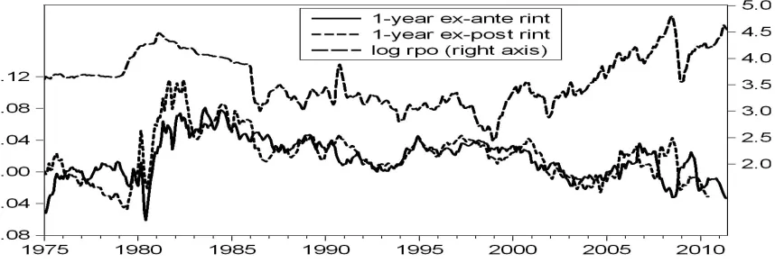
To get a better idea of the relationship between the real oil price and real interest rate, Figure 1 shows the real oil price and ex-post and ex-ante 1-year real interest rates over the sample period. The two measures of the real interest rate do move together over the sample period, but there are clear divergences. In terms of statistics, the mean value of the ex-ante rate is 0.019 while that of the ex-post rate is 0.021. The ex-post rate also has a higher standard deviation, with a value of 0.031 compared with 0.025 for the ex-ante rate. The correlation between the two series is just below 75%. With respect to these rates and the real oil price, there does not seem to be a clear inverse relation between the series over the entire sample period. However, there are periods when such a relationship does exist, such as 1980-1985 or most of the post-2000 period (for the ex-ante rate). Interestingly, the correlation between the real oil price and ex-ante rate is -0.113, while that between the real oil price and ex-post rate is 0.167. It seems that an inverse relation may exist, but may not hold over all periods, and may depend on how the real interest rate is calculated.14
3
Results
The results show that the inverse response of the real oil price to real interest rate innovations depends on the calculation of the real interest rate, the maturity of the rate used, and the ordering of variables. There is a statistically significant inverse response of the real oil price to an innovation in the ex-ante rate, at any maturity. In the ex-post case, this only exists when the short-term rate is used.15
The percent of the forecast error variance of the real oil price accounted for by the real interest rate at any horizon is much larger when shorter-term rates are used. In addition, the sample size can change this response when using longer-term real interest rates. The sample must go through at least 2006 for the real oil price to respond inversely to a long-term real interest rate
11
The corresponding one-month LIBOR rate gives similar results, but is not used because it is not publicly available. Additionally, the yield on three-month U.S. Treasury Bills at constant maturity and ten-year yields on U.S. Treasury Notes at constant maturity are used for robustness as well.
12See
http://www.clevelandfed.org/research/data/inflation_expectations/index.cfmfor more information.
13
Seehttp://www.treasury.gov/resource-center/data-chart-center/tic/Documents/shlhistdat.html.
14
As in Akram (2009), co-integration tests give conflicting results for each of the real interest rate series with respect to the real oil price.
15
innovation. The ordering changes the responses, but the results are robust to the frequency of the data, lag length, time trends, filtering, and additional explanatory variables.
3.1 Baseline
The baseline simulations use a four variable VAR ordered as ip, rint, rex, and rpo. The sample period ranges from 1975-2011M06, the data is of a monthly frequency, each variable save the real interest rate is in logs, and there are 12 lags. The real interest rate is the ex-ante 1-year rate. We use monthly data because it makes interpretation of the ordering easier. In particular, oil prices are less likely to impact the real interest rate over a month, as opposed to one quarter or year. We also assume that industrial production cannot be contemporaneously affected by any of the other variables. Using one year’s worth of data allows for the incorporation of seasonal impacts, which are particularly important for the oil price. There is also evidence that changes in the oil price can take up to a year to impact output (Hamilton and Herrera,2004). Extensions and modifications are considered below.
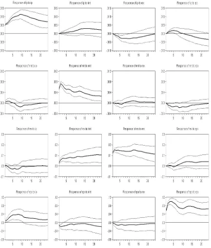
Figure 2 displays all impulse responses from the VAR in the baseline case. The variable being shocked is the same in each column, and the rows have the variables responding to the shock. For example, the first column has the impulse response of each variable in the system to an innovation in industrial production. The dashed lines correspond to plus or minus two standard errors around the impulse responses. Our primary interest is in the response of the real oil price to an innovation in the real interest rate. This can be found in the bottom row, second column. The plot shows that the real oil price falls instantaneously given an innovation in the real interest rate, as we would expect, and the response is statistically significant. At least in the baseline case, there seems to be an inverse relation.16
Other impulse responses move as expected as well. The first column of the bottom row shows that an innovation in industrial production raises the real price of oil. This is consistent with the view that higher demand will raise the oil price. Similarly, the first column of the first row shows that industrial production is persistent, as is well known. Finally, the last column of the bottom row shows that the real oil price is persistent as well.
Variable 1M 4M 1Y 2Y
Industrial Production 1.50 5.02 12.00 9.49 Real Interest Rate 3.94 2.96 1.72 2.17 Real Exchange Rate 0.70 0.82 1.23 1.13 Real Oil Price 94.48 91.21 85.03 87.21
Table 1: Percent of horizon step ahead forecast error variance of the real oil price accounted for by the listed variables. The results are from a four variable VAR, all variables save the real interest rate are in logs, frequency is monthly, and there are 12 lags.
Table 1 shows the variance decomposition of the real oil price for the baseline simulation. The largest fraction of the error variance is accounted for by the real oil price itself, at any of the listed horizons. Industrial production does impact this variance, but the magnitude gradually builds up,
16Granger causality tests between the variables vary depending on whether the ex-post or ex-ante real interest rate
peaking at one year. The real exchange rate has very little effect on the forecast error variance of the real oil price. The real interest rate accounts for almost four percent of the forecast error variance at the one-month horizon, which is instantaneous in our case. But its importance declines over time. Interestingly, at the one-month horizon the real interest rate accounts for more of the error variance than either the real exchange rate or industrial production. We can conclude that in the baseline case rpo does respond inversely to movements in rint, but the magnitude of that impact is limited, especially after one month. Next, I focus on the calculation of the real interest rate.
3.2 Variations in Real Interest Rate
3.2.1 Calculation
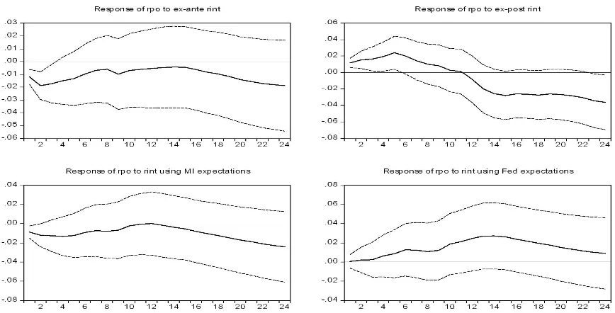
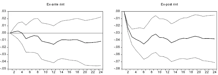
Figure 3 plots the impulse responses of rpo to innovations in ex-ante and ex-post rint (top row), and it also shows these same responses when rint is calculated using inflation expectations from the consumer survey of the University of Michigan, and inflation expectations from the Federal Reserve Bank of Cleveland (bottom row). It seems the response of rpo depends crucially on the method ofrintcalculation. The top left panel repeats the baseline simulation, and shows there is a statistically significant fall inrpowith a positive innovation inrint. This disappears in the ex-post case, as shown in the top-right. Here, rpo rises in the face of a positive innovation to rint. The response ofrpowhenrintis calculated using inflation expectations from the University of Michigan consumer survey is consistent with the baseline, as it falls with the rint innovation. But this also disappears in the bottom left panel with inflation expectations from the Cleveland Federal Reserve are used.
Calculation 1M 4M 1Y 2Y Ex-Ante 3.94 2.96 1.72 2.17 Ex-Post 4.00 3.30 3.43 9.63 MI 1.90 1.48 0.98 2.24 Fed 0.01 0.13 2.16 4.33
Table 2: Percent of horizon step ahead forecast error variance of the real oil price accounted for by the one-year real interest rate under various scenarios. In all cases the results are from a four variable VAR, all variables save the real interest rate are in logs, frequency is monthly, and there are 12 lags.
3.2.2 Term
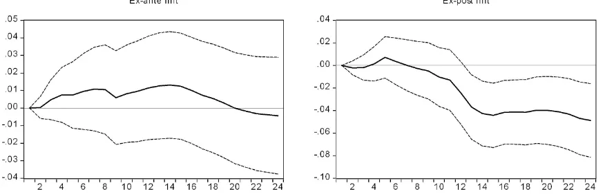
Figure 4 plots the impulse responses of the ex-ante and ex-post real interest rates when the time to maturity is one month.17
When compared with the top row of Figure 3, Figure 4 shows the term of the real interest rate is important in determining the response of rpo to innovations in rint.18
With either the short or long-term rate, there is a fall in rpowith a positive innovation to ex-ante rates. The difference comes with ex-post rates, which continue to show the inverse relation with the short-term rate but not the long-term one.
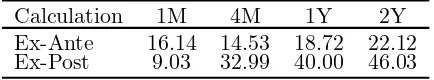
Calculation 1M 4M 1Y 2Y Ex-Ante 16.14 14.53 18.72 22.12 Ex-Post 9.03 32.99 40.00 46.03
Table 3: Percent of horizon step ahead forecast error variance of the real oil price accounted for by the 3-month real interest rate under various scenarios. In all cases the results are from a four variable VAR, all variables save the real interest rate are in logs, frequency is monthly, and there are 12 lags.
Table 3 highlights the importance of the term of rint for the variance decompositions. The instantaneous magnitude of the forecast error variance ofrpo accounted for byrint in the ex-ante case is four times larger with a short-term rate (first row of Table 2 versus the first row of Table 3). The importance increases as the horizon extends over two years. The ex-post results show even larger differences (second row of Table 2 versus the second row of Table 3). At the one-month horizon, the fraction of the forecast error variance of rpo accounted for by rint is twice as large as in the one-year case. This increases to be over five times as large by the two-year mark. These results demonstrate that the term of the real interest rate is an important factor in the relationship betweenrpo andrint.
3.3 Time Variation
Frankel(2006) found that the real oil price responded inversely to movements in U.S. real interest rates in the 1970s, but not into the 1980s and 1990s. This suggests that the relationship may be time-varying, and we consider this by modifying our sample size. Figures 5 and 6 show the impulse responses of the real oil price to the ex-ante one-year and one-month real interest rates under various sample sizes.19
In Figure 5, the left panel shows the response of rpo to ex-ante one-year
rint if the sample ranges from 1975-1999M12, the center shows the response for a sample from 1975-2006M12, and the right panel shows the full sample. In Figure 6, the left panel shows the response of rpo to ex-ante one-year rint if the sample ranges from 1975-1988M12, and the right panel has the full sample.
Figure 5 shows that through 1999, the one-year ex-ante real interest rate does not significantly impact the real oil price. We choose to begin in 1999 because the impulse responses of samples which end before 1999 show similar patterns. These earlier samples also have a similar percent of
17
Inflation expectations are only available from either source for the annual case or longer, so are omitted in this section.
18
The impulse responses of the 3-month rate are similar.
the forecast error variance ofrpo accounted for by rint. Table 4 shows that this begins to change after 1999.
Calculation 1999 2000 2001 2002 2003 2004 2005 2006 1M Response 0.44 0.55 0.88 0.92 1.05 1.29 1.31 1.97
Table 4: Percent of horizon step ahead forecast error variance of the real oil price at one month accounted for by the one-year real interest rate over different sample sizes. In all cases the results are from a four variable VAR, all variables save the real interest rate are in logs, frequency is monthly, and there are 12 lags.
The table shows that after 1999 the percent of forecast error variance of rpo accounted for by the one-year ex-anterint at the one-month horizon gradually rises. It reaches almost two percent when the sample goes through 2006, and the center panel of Figure 5 shows that this is the point where the impulse response of the real oil price has a statistically significant inverse response to a real interest rate innovation. The response of the real oil price becomes stronger as the sample is extended, as shown in the right panel of Figure 5. The results indicate that something changes with respect to the relationship between the real oil price and longer-term U.S. real interest rates after 1999.
Figure 6 shows that the real oil price has responded inversely to innovations in shorter-term U.S. real interest rates since 1988.20 We interpret this as showing that the relationship betweenrpo
and short-term rates has been relatively stable over time. This indicates that the behavior of those who store oil has been relatively consistent, and is very responsive to short-term U.S. real interest rates. We conclude thatrpohas consistently responded inversely to innovations in short-termrint, but has only recently done so for longer-term rint. We turn next to the ordering in our recursive VAR.
3.4 Ordering
As discussed in Cochrane (1994), the choice of ordering has important implications when using a recursive VAR. To gauge its importance, we modify our ordering in both the ex-ante and ex-post cases for short and long-term rates. Figure 7 shows the impulse responses ofrpoover the full sample to both the ex-ante and ex-post one-year real interest rates when the ordering is: ip,rpo,rex, and
rint.21 Figure 8 shows the same for the one-month real interest rate. Changing the ordering also
changes the interpretation of the impulse responses. Because rint can no longer instantaneously impactrpo, it might still be the case that there is an inverse relation, but it is being overshadowed by something else. However, the existence of the inverse response in this case can demonstrate the strength of the relationship.
For the one-year rate, Figure 7 shows that modifying the ordering changes the results substan-tially. In particular, rpo no longer falls with a positive innovation in either the ex-ante or ex-post one-year rate. Although not statistically significant, the ex-ante calculation shows a rise in the real oil price, while the ex-ante case still falls. The responses ofrpoto innovations in the one-monthrint
are mixed with this alternative ordering. The left panel of Figure 8 is consistent with the long-term
20
Although not true before 1988, it may be due to the small sample size if looking earlier than this date.
21
case, as the ex-ante rate does not induce a statistically significant fall in the real oil price. The ex-post rate, however, does induce a statistically significant inverse response. We conclude that the short-term rates have a stronger relationship withrpothan longer-term rates, given the possibility the relationship still holds under the alternative ordering. In our final section, we further check the robustness of our results.
3.5 Other Variations
Here, we modify the baseline simulation by varying the lag length, changing the frequency of the data, adding a linear trend, filtering, differencing the real oil price, and adding additional explanatory variables. The baseline response of rpo to innovations in rint is not sensitive to the lag length used. In this case, the Akaike information criterion selects a minimum lag length of four months, as does the final prediction error. However, a lag length of 12 months was chosen to incorporate both seasonal impacts and the lagged responses of industrial production and other variables to changes in the real oil price, as discussed inHamilton and Herrera (2004). Still, both impulse responses and variance decompositions using a lag of four months are similar to the twelve month case.
The frequency of the data does not change the relation either in the baseline case. Using quar-terly instead of monthly data can vary individual impulse responses and variance decompositions in terms of magnitude, but the directions (and statistical significance) are similar to the baseline case. The same is true of adding a deterministic trend or filtering the data using the HP filter. There is some evidence that oil prices contain an explosive componentShi and Arora(2011). Using the log difference of the oil price instead of the log itself also does not make a difference to our baseline results. The inverse relationship is also robust to adding additional explanatory variables. For example, OPEC spare production capacity is often considered an important determinant of the real oil price. Adding this data to the VAR (in any ordering) does not alter the relation between
rpoand rint. We also added OPEC production, total world oil production and found the same to be true in these cases as well.
4
Conclusions and Future Work
Consistent with theory, the real oil price does respond inversely to movements in the real interest rate. However, the robustness and magnitude of this movement depends on characteristics of the real interest rate. The first is in how the real interest rate is calculated. Longer-term real interest rates cannot generate an inverse response in the real oil price if the calculation is ex-post. This is not true for shorter-term rates, which are robust to the method of calculation. The response of the real oil price to short-term rates also does not vary over time, but does so with long-term rates. For the real oil price to respond inversely to long-term rates, the sample must run through at least 2006. Finally, innovations in ex-post short-term rates still lead to an inverse response in the real oil price under alternative orderings.
rates, this provides a direct channel whereby monetary actions can have direct (and real) impacts on the oil price. An interesting question is the relative importance of monetary policy changes for oil price variation through this channel.
The impact of long-term real interest rates on the real oil price is more difficult to explain. One possible explanation is that oil producers have started treating oil in the ground more like a conventional asset. This may be due to the proliferation of sovereign wealth funds in oil producing countries, which lead them to treat oil in the ground more like an asset class than in the past. If oil producers have changed their behavior, then production should respond to U.S. real interest rate innovations. It could also be the case that only producers with sovereign wealth funds have changed their behavior, while others have not. In this case the response of oil production to the same innovations should differ by country.
Another possible explanation for the response of oil prices to longer-term real interest rates is based on portfolio reallocation and the increased financialization of commodity markets. Facing low (and falling) U.S. real interest rates, investors have moved out of other assets and into commodities, particularly oil futures, resulting in higher prices. Alternatively,Buyuksahin et al.(2008) find that there was a structural change in the relation between crude oil futures prices across a range of maturities in the early 2000s. The observations with longer-term rates may just be a manifestation of this change.This may help to explain the increased response of oil prices to longer-term rates as well.
References
Akram, Q. Farooq, “Commodity Prices, Interest Rates and the Dollar,” Energy Economics, 2009, 31, 838–851.
Alquist, Ron, Lutz Kilian, and Robert J. Vigfusson, “Forecasting the Price of Oil,” in G. Elliott and A. Timmermann, eds., Prepared for The Handbook of Economic Forecasting, 2nd ed., North-Holland, 2011.
Anzuini, Alessio, Marco J. Lombardi, and Patrizio Pagano, “The Impact of Monetary Policy Shocks on Commodity Prices,” Working Paper 1232, European Central Bank 2010.
Arora, Vipin, “Asset Value, Interest Rates, and Oil Price Volatility,”The Economic Record, 2011,
87 (s1), 45–55.
and Rod Tyers, “Asset Arbitrage and the Price of Oil,” Economic Modelling, 2011, Forth-coming.
Belke, Ansgar, Ingo G. Bordon, and Torben W. Hendricks, “Global Liquidity and Com-modity Prices - A Cointegrated VAR Approach for OECD Countries,” Applied Financial
Eco-nomics, 2010,20, 227–242.
Buyuksahin, Bahattin, Michael S. Haigh, Jeffrey H. Harris, James A. Overdahl, and Michael A. Robe, “Fundamentals, Trader Activity and Derivative Pricing,” 2008.
Deaton, Angus and Guy Laroque, “On the Behaviour of Commodity Prices,”Review of
Eco-nomic Studies, 1992,59 (1), 1–23.
Frankel, Jeffrey A., “Expectations and Commodity Price Dynamics: The Overshooting Model,”
American Journal of Agricultural Economics, 1986, 68(2), 344–348.
, “The Effect of Monetary Policy on Real Commodity Prices,” Working Paper 12713, NBER 2006.
and Andrew K. Rose, “Determinants of Agricultural and Mineral Commodity Prices,” in “Inflation in an Era of Relative Price Shocks” Reserve Bank of Australia August 2009.
Hamilton, James and Ana Maria Herrera, “Oil Shocks and Aggregate Macroeconomic Be-havior: The Role of Monetary Policy,” Journal of Money, Credit and Banking, 2004, 36 (2), 256–286.
Hamilton, James D., “Understanding Crude Oil Prices,” The Energy Journal, 2009, 30 (2), 179–206.
Hotelling, Harold, “The Economics of Exhaustible Resources,” Journal of Political Economy, 1931, 39, 137–175.
Krichene, Noureddine, “World Crude Oil Markets: Monetary Policy and the Recent Oil Shock,” Working Paper WP/06/62, IMF 2006.
Reicher, Christopher P. and Johannes Utlaut, “The Relationship Between Oil Prices and Long-Term Interest Rates,” Working Paper 1637, Kiel Institute for the World Economy 2010.
Shi, Shuping and Vipin Arora, “An Application Of Models Of Speculative Behaviour To Oil Prices,” Working Paper 2011-11, CAMA 2011.
Slade, Margaret E. and Henry Thille, “Wither Hotelling: Tests of the Theory of Exhaustible Resources,” Annual Review of Resource Economics, 2009, 1, 239–259.
Tang, Ke and Wei Xiong, “Index Investing and the Financialization of Commodities,” Working Paper 2009.
Working, Holbrook, “The Theory and Price of Storage,”The American Economic Review, 1949,
39 (6), 1254–1262.
Figure 3: Responses (percent change) of the real oil price to a one standard deviation innovation in various 1-year real interest rates, 1975-2011M06. Top Left: Ex-ante rate; Top Right: Ex-post rate; Bottom Left: Rate using Michigan inflation expectations; Bottom Right: Rate using Cleveland Fed inflation expectations. The dashed lines are +/- two standard errors.
[image:17.612.95.521.455.601.2]Figure 5: Responses (percent change) of the real oil price to a one standard deviation innovation in the ex-ante one-year real interest rate. Left: 1975-1999; Center: 1975-2006; Right: 1975-2011M06. The dashed lines are +/- two standard errors.
Figure 6: Responses (percent change) of the real oil price to a one standard deviation innovation in the ex-ante one-month real interest rate. Left: 1975-1988; Right: 1975-2011M06. The dashed lines are +/- two standard errors.
[image:18.612.89.527.491.632.2]