Temporal Causality and the Dynamics of Crime in Turkey

(1)

Munich Personal RePEc Archive

Temporal Causality and the Dynamics of

Crime in Turkey

Halicioglu, Ferda

Department of Economics, Yeditepe University

2012

Online at

https://mpra.ub.uni-muenchen.de/41794/

(2)

This study is concerned with understanding of the factors of aggregate, nonviolent and violent

crime categories in Turkey for the period 1965 2009. The determinants of all crime categories

are related to selected socio economic factors. Bounds testing approach to cointegration is

employed to test the existence of long run relationship amongst the variables. Cointegration

analysis yields the major contributors of crime are income and unemployment. The direction

of causalities between the variables are established using within and out of sample causality

tests. The findings from this study present the dynamics of aggregate, violent and non violent

crimes to design and implement any relevant policy measures to combat them.

crime, cointegration, causality, time series, Turkey C22, A14, K42

! !"# $

Department of Economics, Yeditepe University, Istanbul,

34755 Turkey

(3)

!% !

The theoretical and empirical work on the socio economic determinants of crime has grown

substantially since the seminal study of Becker (1968), which suggests that the criminal

behaves in a rational way and decides how to allocate time between legitimate and

illegitimate activities, based on an income benefit cost comparison, plus the likelihood of

apprehension and conviction.

Crime is a universal problem which has a detrimental effect on the functioning and stability of

society. Moreover, prevention of crime is always a major public policy concern for all

countries due to its socio economic implications and costs. The extent of crimes may vary

from country to country. However, a recent study of Harrendorf et al. (2010) provides some

comparable international crime statistics based on the police records in homicide, assault,

rape, robbery, burglary, motor vehichle theft and kidnapping rates for 144 countries. All crime

rates are reported below per 100,000 population. As of 2004, approximately 490,000 deaths

from international homicide occured revealing the rate of 7.6. In the same year, there were

4973 Turkish homicides, which produced the homicide rate of 7.07. As of 2006, the mean

assault rate in the world was 251 whilst it was 192.7 in Turkey. Considering rape rates, the

mean world rape rate was 12 but Turkey had a substantially low rape rate value of 2.5. Even

though Harrendorf et al. (2010) reports individually the mean robbery rates for 144 countries

but the mean value was not presented. The robbery rate for Turkey was revealed as 28.3

which was classified as low. The mean burglary rate for the world was illustrated as 339

whereas Turkey had a burglary rate of 216.9. As for the mean motor vehicle theft rates,

Turkish rate, 45.9 is well below of the world average of 118. Finally, the kidnapping rates

were compared, according to this rate, Turkey ranked the top with a rate of 14.84 whereas the

(4)

The international crime statistics demonstrate that the crime rates in Turkey apart from the

kidnapping rates are below the world averages indicating low occurance of criminal

activities. The crime rates in Turkey, nevertheless, seem to be on surge considering the data

provided by Turkish Institute of Statistics (TSI), as of January 2011, there were 66997

convicts in the Turkish prisons which convert as 91.52 conviction per 100,000 population and

the Turkish prisons are overflowed by the number of convicts and the people arrested waiting

for trials, currently 55407. However, it should be noted that an increase in conviction rate may

not be directly imply a rise in crime activities as the extent and definitions of crime categories

may be modified considerably regarding the crime time series data.

An empirical study of crime in Turkey may provide useful policy tools for the policy makers

to predict the future development on aggregate, violent and nonviolent crimes. The

development in crime is a crucial factor in demands which are placed on the police and the

criminal justice system. The empirical studies aiming at determining the causes of crime in

Turkey are limited. For example, Kustepeli and Onel (2006) applies Johansen Juselius (1990)

cointegration approach to identify the determinants of crime using annual data of 1967 2004

but it is well documented the adopted cointegration methodology is strictly for large samples.

Therefore, the results from Kustepeli and Onel (2006) are considered as flawed. The study of

Comertler and Kar (2007) on crime is based on cross section data, as a result it lacks of

direction of causations between the variables. As far as this study is concerned, there exists no

previous study that estimates empirically the determinants of crime in Turkey implementing

the cointegration framework of Pesaran et al. (2001). Thus, this study aims at contributing to

the existing literature by providing fresh evidence on the determinants of crime in addition to

(5)

It is expected that the results from this study will have also some implications for the

countries which are in the same development stage of Turkey. The extensions and

modifications of the model presented here may also contribute to the enrichment of the

existing literature on quantitative crime studies.

The remainder of this paper is organized as follows. Section 2 presents a brief literature

review. Section 3 describes the study’s model and methodology. Section 4 discusses the

empirical results, and finally Section 5 concludes.

!!% &

Ehrlich (1973) further extended the research of Becker (1968) on crime and introduced initial

econometrics model of offences. Ehrlich (1996) outlines the main themes of the literature on

crime. The existing literature in crime economics divides the variables affecting the crime rate

broadly into three categories: economic, socioeconomic demographic, and deterrent.

There are two most frequently used economic variables that are linked to criminal activities,

unemployment and income. Cantor and Land (1985) proposed that there are two distinct and

potentially counter balancing mechanisms which unemployment may affect crime rates in the

aggregate: motivation and criminal opportunity. Former approach relates unemployment to

crime rates positively in which a rise in unemployment leads to economic problems and

increases the motivation to engage in criminal acts, see for example Reilly and Witt (1992)

and Edmark (2005). Latter approach sets up an inverse relationship between these two

variables indicating that economic deprivation leads reduction in the supply of worthwhile

targets for the criminals. A variant of the latter approach also suggests that a rise in

unemployment rates leads to decrease in median family income and discourages a person

(6)

between income and crime is formed through three different ways. First an income decrease

causes the need for returns from illegal activities; see for example Machin and Meghir (2000).

Second an income increase sets the opportunities for criminal activities due to the large

amount of stolen goods as pointed out in Lewitt (1999). Third a rise in income leads to

outdoor activities, which stimulates potential crime activities, as discussed in Beki et al.

(1999). This impact may occur in reverse order if a rise in income leads to a decrease in

unemployment which alleviates the need for crime. As for the socioeconomic demographic

determinants of crime, urbanization appears to be one of key explanatory factor with an

implication that it causes an increase in criminal activities, see for example Masih and Masih

(1996). According to Gartner (1990), the rate of divorce is related to criminal activities as

such that changing guardianship and the members of disturbed families pose risk everyone in

the society. The impact of deterrent variables such as the number of police force or security

expenditures, conviction rates, arrests on crime appear to be usually positive apart from some

crime categories since they do not always lead to conviction or arrest, see for example

Corman et al. (1987).

There is a very large and growing body of research on different categories of crime linking

them with a number of socio economic determinants. Soares (2004) provides an extensive

survey of the empirical studies on crime rates based on 40 studies. An earlier survey of

Chiricos (1987) especially presents detailed evidence on the relationship between crime and

unemployment rates from 63 research articles.

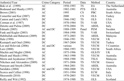
Table 1 reveals that the empirical studies on crime is based on a number of different

empirical methods ranging from simple correlation to sophisticated panel econometric

procedures with different categories of crime applying cross section to time series data. The

(7)

researchers indicating the diversity of the empirical evidence on crime. The recent studies

[image:7.595.44.566.137.476.2]

usually tend to apply cointegration framework and time series data.

Table 1. Summary results of the selected empirical works on crime

Author(s)/Year Crime Category Period Data Method Country

Beki et al . (1999) AC 1950 1993 TS EG The Netherlands

Bodmand and Maulty (1997) DC 1982 1991 PTS OLS Australia

Brown (2001) AC 1995 CS PBC South Africa

Comertler and Kar (2007) DC 2000 CS OLS Turkey

Canton and Land (1985) DC 1946 1982 TS OLS USA

Corman et al. (1987) DC 1970 1984 TS VAR USA

Detotto and Pulina (2009) DC 1970 2004 TS ARDL Italy

Edmark (2005) AC and DC 1988 1999 Panel PEM Sweden

Funk and Kugler (2003) DC 1984 1998 TS VAR Switzerland

Habibullah and Baharom (2009) DC 1973 2003 TS ARDL Malaysia

Hale (1998) DC 1946 1991 TS VECM UK

Kustepeli and Onel (2006) DC 1967 2004 TS VECM Turkey

Lee and Holoviak (2006) AC and DC various TS VECM 5 Countries

Luiz (2000) DC 1960 1993 TS VECM South Africa

Machin and Meghir (2004) AC 1975 1996 TS OLS/IV UK

Masih and Masih (1996) DC 1963 1990 TS VECM Australia

Meera and Jayakumar (1995) DC 1968 1988 TS TSLS Malaysia

Nikolaos and Alexandros (2009) AC 1971 2006 TS VECM Greece

Narayan and Smyth (2004) DC 1964 2001 TS ARDL Australia

Saridakis (2004) AC and DC 1960 2000 TS VECM USA

Scorcu and Cellini (1998) DC 1951 1994 TS ECM Italy

Shoesmith (2010) DC 1970 2003 TS VECM USA

Reilly and Witt (1992) DC 1974 1988 TS OLS Scotland

Keys: AC (Aggregate Crime), DC (Disaggregate Crime), EG (Engle Granger), CS (Cross Section), TS (Time Series), PTS (Pooled Time Series), Likelihood), OLS (Ordinary Least Squares), PBC (Pearson Pairwise Correlation), IV (Instrumental Variables), TSLS (Two Stage Least Squares), ECM (Error Correction Model), PEM (Panel Econometric Methods), VAR (Vector Auto Regression), ARDL (Auto Regressive Distributed Lag), VECM (Vector Error Correction Model).

!!!% ' (

Following the empirical literature on crime, this study adopts the following long run

relationship between crime, income, unemploymet, divorce, urbanization and security

expenditures in double linear logarithmic form as:

t t t

t t

tj a a y au ad a r a s

(8)

where the subscript t indexes time period with t =1965,…, 2009; ct is convicts per 100,000

people; j indexes convict variable with j=0 (aggregate crime is the combination of nonviolent

and violent offences), 1 (nonviolent crime consist of property, burglary, motor vehicle theft,

fraud, corruption, etc.), and 2 (violent crime includes homicide, assault, rape, and

kidnapping); yt is real income per capita; ut is unemployment rate; dt is divorce rate per

1000; rt is urbanization rate; st is real public security expenditures per capita; and

ε

t is the

classical error term.

Cointegration

Recent advances in econometric literature dictate that the long run relation in equation (1)

should incorporate the short run dynamic adjustment process. It is possible to achieve this aim

by expressing equation (1) in an error correction model as suggested in Pesaran et al. (2001).

t t t t j t t j t n i i t i n i i t i i t n i i n i n i n i i t i i t i j i t j i j t v s r d u y c s r d u y c c + + + + + + + + + + + + + = − − − − − − = − = − − = = − = − = −

∑

1 12 1 11 1 10 , 1 9 1 8 , 1 7 6 0 6 5 0 5 4 0 4 1 1 2 0 3 0 3 2 , , 1 0 , β β β β β β β β β β β β β (2)

This approach, also known as autoregressive distributed lag (ARDL), provides the short run

and long run estimates simultaneously. Short run effects are reflected by the estimates of the

coefficients attached to all first differenced variables. The long run effects of the explanatory

variables on the dependent variable are obtained by the estimates of β8 β12 that are normalized

on β7. The inclusion of the lagged level variables in equation (2) is verified through the

bounds testing procedure, which is based on the Fisher (F) or Wald (W) statistics. This

procedure is considered as the pre testing stage of the ARDL cointegration method.

(9)

0

12=

β

), against the alternative hypothesis, (H1: at least one of

β

7 to

β

12≠0) should be

performed for equation (2). The F/W test used for this procedure has a non standard

distribution. Thus, Pesaran et al. (2001) compute two sets of critical values for a given

significance level with and without a time trend. One set assumes that all variables are I(0)

and the other set assumes they are all I(1). If the computed F/W statistic exceeds the upper

critical bounds value, then the H0 is rejected, implying cointegration. In order to determine

whether the adjustment of variables is toward their long run equilibrium values, estimates of

β7 β12 are used to construct an error correction term (EC). Then lagged level variables in

equation (2) are replaced by ECt 1 forming a modified version of equation (2) as follows:

t t n i n i i t i i t i i t n i i n i n i n i i t i i t i j i t j i j t EC s r d u y c c λ α α α α α α α + + + + + + + + = − = − = − − = = = = − − −

∑

1 5 0 6 0 6 5 4 0 4 1 1 2 0 3 0 3 2 , , 1 0 . (3)

Equation (3) is re estimated one more time using the same lags previously. A negative and

statistically significant estimation of λ not only represents the speed of adjustment but also

provides an alternative means of supporting cointegration between the variables. Pesaran et

al. (2001) cointegration approach has some methodological advantages in comparison to other

single cointegration procedures. Reasons for the ARDL are: i) endogeneity problems and

inability to test hypotheses on the estimated coefficients in the long run associated with the

Engle Granger (1987) method are avoided; ii) the long and short run coefficients of the model

in question are estimated simultaneously; iii) the ARDL approach to testing for the existence

of a long run relationship between the variables in levels is applicable irrespective of whether

(10)

cointegrated; iv) the small sample properties of the bounds testing approach are far superior to

that of multivariate cointegration, as argued in Narayan (2005).

Augmented Granger Causality

The Granger representation theorem suggests that there will be Granger causality in at least

one direction if there exists a cointegration relationship among the variables in equation (1),

providing that they are integrated order of one. Engle and Granger (1987) caution that the

Granger causality test, which is conducted in the first differenced variables by means of a

VAR, will be misleading in the presence of cointegration. Therefore, an inclusion of an

additional variable to the VAR system, such as the error correction term would help us to

capture the long run relationship. To this end, an augmented form of the Granger causality

test involving the error correction term is formulated in a multivariate pth order vector error

correction model.

[

]

                    +                     +                                         − +                     =                     − ₋ − − − − − − =

∑

t t t t t t t i t i t i t i t i t i tj i i i i i i i i i i i i p i t t t t t tj EC s r d u y c L s r d u y c L 6 5 4 3 2 1 1 6 5 4 3 2 1 66 61 56 51 46 ' 41 36 31 26 21 16 11 1 6 5 4 3 2 1 ..., ,... ..., ,... ., ... ,... ..., ,... ..., ,... ..., ,... ) 1 ( ) 1 ( ω ω ω ω ω ω δ δ δ δ δ δ φ φ φ φ φ φ φ φ φ φ φ φ θ θ θ θ θ θ (4) ) 1

( −L is the lag operator. ECt 1 is the error correction term, which is obtained from the long

run relationship described in equation (1), and it is not included in equation (4) if one finds no

cointegration amongst the vector in question. The Granger causality test may be applied to

equation (4) as follows: i) by checking statistical significance of the lagged differences of the

(11)

statistical significance of the error correction term for the vector that there exists a long run

relationship. As a passing note, one should reveal that equation (3) and (4) do not represent

competing error correction models because equation (3) may result in different lag structures

on each regressors at the actual estimation stage; see Pesaran et al. (2001) for details and its

mathematical derivation. All error correction vectors in equation (4) are estimated with the

same lag structure that is determined in unrestricted VAR framework.

Variance Decompositions

Establishing Granger causality is restricted to essentially within sample tests, which are

useful in distinguishing the plausible Granger exogeneity or endogenity of the dependent

variable in the sample period, but are unable to deduce the degree of exogenity of the

variables the beyond the sample period. To examine this issue, the decomposition of variance

of the variables may be used. The variance decompositions (VDCs) measure the percentage of

a variable’s forecast error variance that occurs as the result of a shock (or an innovation) from

a variable in the system. The VDCs estimate the percentage contribution of each variable

including the dependent variable in the total variation of the dependent variable. Sims (1980)

notes that if a variable is truly exogenous with respect to the other variables in the system,

own innovations will explain all of its forecast error variance (i.e., almost 100%). By looking

at VDCs policy makers gather additional insight as to what percentage (of the forecast error

variance) of each variable is explained by its determinant.

(12)

Annual data over the period 1965 2009 were used to estimate equation (2) and (3) by the

ARDL cointegration procedure of Pesaran et al. (2001). Variable definition and sources of

data are cited in Appendix.

To implement the Pesaran et al. (2001) procedure, one has to ensure that none of the

explanatory variables in equation (1) is above I(1).In the presence of I(2), the critical values

computed by the Pesaran et al. (2001) cointegration procedure are not valid. Three tests were

used to test unit roots in the variables: Augmented Dickey Fuller (henceforth, ADF) (1979,

1981), Phillips Perron (henceforth, PP) (1988), and Elliott Rothenberg Stock (henceforth,

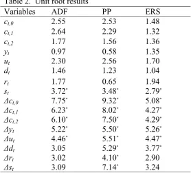
ERS) (1996). Unit root tests results are displayed in Table 2. Table 2 demonstrates that none

of the variables included in the model are beyond I(1). Consequently, the results warrant

implementing the Pesaran et al. (2001) procedure. Visual inspections of the variables in

[image:12.595.158.437.422.673.2]

logarithm show no structural breaks.

Table 2. Unit root results

Variables ADF PP ERS

ct,0 2.55 2.53 1.48

ct,1 2.64 2.29 1.32

ct,2 1.77 1.56 1.36

yt 0.97 0.58 1.35

ut 2.30 2.56 1.70

dt 1.46 1.23 1.04

rt 1.77 0.65 1.94

st 3.72* 3.48* 2.79*

!ct,0 7.75* 9.32* 5.08*

!ct,1 6.23* 8.02* 4.27*

!ct,2 6.10* 7.50* 4.29*

!yt 5.22* 5.50* 5.26*

!ut 4.46* 5.51* 4.47*

!dt 3.05 5.29* 3.77*

!rt 3.02 4.10* 2.90

!st 3.09 7.14* 3.24

(13)

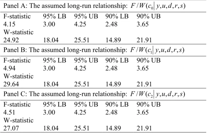
In order to test the existence of a long run cointegrating relationship amongst the variables of

equation (1), a two step procedure to estimate the ARDL representation model was carrried

out. First, in search of the optimal lag length of the differenced variables of the short run

coefficients in equation (2), unrestricted Vector Auto Regression (VAR) was employed by

means of Akaike Information criteria (AIC). The results suggest the optimal lag length for all

crime models is 2, but this stage of the results is not presented here to conserve space. Second,

a bound F/W test was applied to equation (2) in order to determine whether the dependent and

independent variables are cointegrated in each crime model. The results of the bounds F/W

testing are reported in Table 3. It can bee seen from Table 3 that the computed F/W statistics

are above the upper bound values in all cases of crime models thus implying cointegration

[image:13.595.65.428.404.635.2]

relations.

Table 3. The results of F and W tests for cointegration.

Panel A: The assumed long run relationship: F/W(c0 y,u,d,r,s)

F statistic 95% LB 95% UB 90% LB 90% UB

4.15 3.00 4.25 2.48 3.65

W statistic

24.92 18.04 25.51 14.89 21.91

Panel B: The assumed long run relationship: F/W(c1 y,u,d,r,s)

4.94 3.00 4.25 2.48 3.65

W statistic

29.64 18.04 25.51 14.89 21.91

Panel C: The assumed long run relationship: F/W(c₂ y,u,d,r,s)

4.51 3.00 4.25 2.48 3.65

W statistic

27.07 18.04 25.51 14.89 21.91

If the test statistic lies between the bounds, the test is inconclusive. If it is above the upper bound (UB), the null hypothesis of no level effect is rejected. If it is the below the lower bound (LB), the null hypothesis of no level effect cannot be rejected.

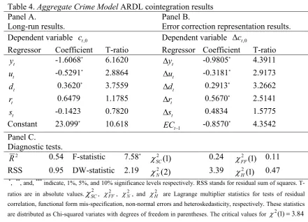
The ARDL representation equation was estimated to obtain the long run and short run

coefficients simultaneously. The results are displayed in Tables 4, 5 and 6, respectively. The

(14)

respectively. The error correction representations from the estimations of equation (3) are

presented in Panel B of Tables 4, 5 and 6, respectively. The stability of coefficients in the

error correction models were also checked via the graphical representations of CUSUM and

CUSUMSQ tests of Brown et al. (1975). The results display that all coefficients in the error

correction models are stable and there exist no structural breaks. These results are not

illustrated here due space considerations.The overall regression diagnostics in all models

suggest that the econometric results are satisfactory to infer from them.. Regarding the

aggregate crime model, in the long run all the parameters seem to be carrying expected signs

but three of them: income, unemployment and divorce rates are statistically and individually

significant. Amongst these variables, income variable has the highest partial impact on crime

indicating that a 1% increase in real per capita income decreases aggregate crime by 1.60% in

the long run. The elasticity of aggregate crime with respect to unemployment rate is 0.53

implying that a 1% rise in the unemployment rate will reduce the criminal opportunities by

0.53%. The impact of unemployment on crime is frequently tested as it is considered as one

of major determinants of crime offenses. Chiricos (1987) for extensive survey linking the

unemployment and crime rates. As for the divorce variable, its affect on the aggregate crime

level is rather noticeable since a 1% increase in divorce rates leads to 0.36% in the aggregate

crime. The short run estimation of the aggregate crime model reveals that the estimated error

correction term is very high ( 0.85) therefore any disequlibrium between the short run and

long run is eliminated within a short period of time. In other words, the aggregate crime

equation is above or below its equilibrium level, it adjusts by 85% within the first year. The

(15)

[image:15.595.60.502.82.400.2]

Table 4. Aggregate Crime Model ARDL cointegration results Panel A.

Long run results.

Panel B.

Error correction representation results. Dependent variable c_t_,₀ Dependent variable c_t_,₀

Regressor Coefficient T ratio Regressor Coefficient T ratio

t

y 1.6068* _6.1620

t

y 0.9805* _4.3911

t

u 0.5291* _2.8864

t

u 0.3181* _2.9173

t

d 0.3620* _3.7559

t

d 0.2913* _3.2662

t

r 0.6479 1.1785

t

r 0.5670* _2.5141

t

s 0.1423 0.7820

t

s 0.4834 1.5775

Constant 23.099* _10.618

1

−

t

EC 0.8570* _4.3542

Panel C.

Diagnostic tests.

2

R 0.54 F statistic 7.58*

χ

_SC2 (1) 0.24

χ

_FF2 (1) 0.11 RSS 0.95 DW statistic 2.19 2₍₂₎

'

χ

3.39 2₍₁₎

H

χ

0.47

*

, **, and, *** indicate, 1%, 5%, and 10% significance levels respectively. RSS stands for residual sum of squares. T ratios are in absolute values.

χ

_SC2 , χ_FF2 , χ2_', and χ_H2 are Lagrange multiplier statistics for tests of residual correlation, functional form mis specification, non normal errors and heteroskedasticity, respectively. These statistics

are distributed as Chi squared variates with degrees of freedom in parentheses. The critical values for χ2(1)=3.84

and χ2(2)=5.99 are at 5% significance level.

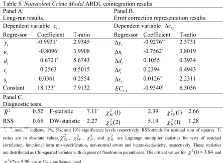
The nonviolent crime model is displayed in Table 5 indicating that income, unemployment

and divorce rate variables are also here statistically and individually significant in the long

run. In fact, the order of their impacts on the dependent variables follow the same order as in

the case of the pervious model but the magnitudes are different. For example, the elasticity of

the nonviolent crime with respect to income is almost 1 impying that there is an exact

proportional change between these variables but it is substantially less in comparison to the

aggregate crime results. The partial impact of unemployment on the nonviolent crime is here

much higher than the previous category of crime. Similarly, the elasticity of the nonviolent

crime is almost twice more than the aggregate crime model. Nevertheless, the error correction

(16)

[image:16.595.65.510.84.410.2]

Table 5. 'onviolent Crime Model ARDL cointegration results Panel A.

Long run results.

Panel B.

Error correction representation results. Dependent variable c_t_,₁ Dependent variable c_t_,₁

t

y 0.9931* _2.9345

t

y 0.9276** _2.3731

t

u 0.8096* _3.9908

t

u 0.7562* _3.8019

t

d 0.6721* _5.6743

t

d 0.1055 0.3934

t

r 0.2563 0.5015

t

r 0.2394 0.4943

t

s 0.0361 0.2554

t

s 0.0126** _2.2311

Constant 18.133* _7.9132

1

−

t

EC 0.9340* _6.3036

Panel C.

Diagnostic tests.

2

χ

_SC2 (1) 2.39

χ

'

χ

5.19 2₍₁₎

H

χ

1.28

*

χ

are distributed as Chi squared variates with degrees of freedom in parentheses. The critical values for χ2(1)=3.84 and

99 . 5 ) 2 (

2 ₌

χ are at 5% significance level.

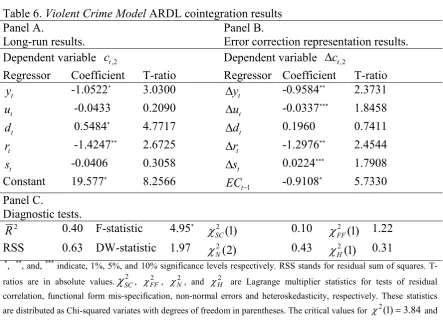
Considering the last category of crime model, even though income and divorce rate variables

are statitically and individually significant as in the case of both previous models. However,

the unemployment variable is not statistically significant in this crime model. Instead,

urbanization variable appears to be statitically significant. The magnitude of the partial impact

of income on the violent crime level is the almost same as the non violent crime in the long

run. The elasticity of violent crime with respect to divorce rate is considerably less than the

nonviolent crime category but substantially higher than the aggregate crime model. It seems

that urbanization is only statistically significant in the case of this category crime. Its

estimated coefficent indicates that a 1% rise in the urbanization rate reduces the violent crime

by 1.42%. As people live close by it is likely that crime rates will drop in comparison to

sparsely located residents. As for the error correction term, its magnitute between the

(17)

[image:17.595.68.512.92.413.2]

Table 6. Violent Crime Model ARDL cointegration results Panel A.

Long run results.

Panel B.

Error correction representation results. Dependent variable c_t_,₂ Dependent variable c_t_,₂

t

y 1.0522* _3.0300

t

y 0.9584** _2.3731

t

u 0.0433 0.2090

t

u 0.0337*** _1.8458

t

d 0.5484* _4.7717

t

d 0.1960 0.7411

t

r 1.4247** _2.6725

t

r 1.2976** _2.4544

t

s 0.0406 0.3058

t

s 0.0224*** _1.7908

Constant 19.577* _8.2566

1

−

t

EC 0.9108* _5.7330

Panel C.

Diagnostic tests.

2

χ

_SC2 (1) 0.10

χ

'

χ

0.43 2₍₁₎

H

χ

0.31

*

χ

are distributed as Chi squared variates with degrees of freedom in parentheses. The critical values for χ2(1)=3.84 and

99 . 5 ) 2 (

2 ₌

χ are at 5% significance level.

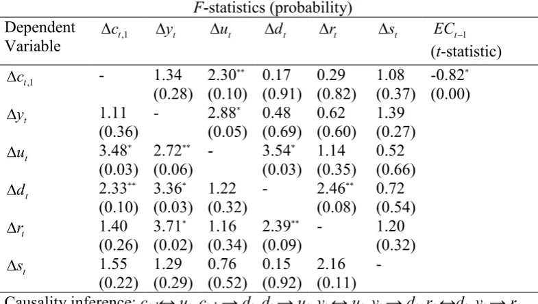
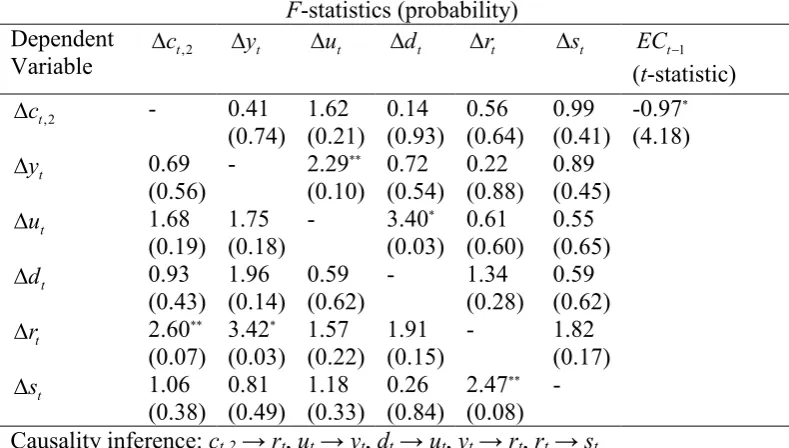
The results of Granger causality tests presented in Tables 7, 8 and 9, respectively, reveal the

existence of the long run causality in the case of each crime categories. In the long run,

causality runs from police expenditures, urbanization, divorce, unemployment and income to

crimes. Howevever, the short run causalities differ amongst the models. Regarding the pairs

of causalities between only crime and explanatory variables, the following points are

identified. There exists a feedback relationship between aggregate crime level and per capita

income. The causality running from crime to per capita income suggests that crime is a

detrimental factor for the economic growth in the short run. Similarly, there is also a feedback

relationship amongst nonviolent crime and unemployment rate. Finally, it is established that a

unilateral causality running from nonviolent crime to divorce rate and violent crime Granger

(18)

[image:18.595.75.465.111.344.2]

Table 7. Results of Granger causality for aggregate crime model F statistics (probability)

Dependent

Variable t,0

c y_t u_t d_t r_t s_t EC_t₋₁

(t statistic)

0 ,

t

c 3.99*

(0.01) 0.62 (0.60) 1.28 (0.30) 0.35 (0.78) 1.17 (0.33) 0.87* (0.02) t

y 3.94*

(0.02) 1.82 (1.16) 1.41 (0.26) 0.88 (0.46) 0.84 (0.48) t u 0.80 (0.50) 0.62 (0.54) 1.16 (0.34) 0.57 (0.63) 0.88 (0.46) t d 0.42 (0.74) 1.39 (0.26) 0.39 (0.26) 1.18 (0.33) 0.38 (0.76) t r 0.13 (0.94) 2.63** (0.07) 0.46 (0.70) 1.29 (0.30) 0.92 (0.44) t s 0.70 (0.55) 0.84 (0.48) 1.27 (0.30) 0.46 (0.70) 1.47 (0.24) Causality inference: ct,0 ↔ yt , yt → rt

*

and ** indicate 5 % and 10 % significance levels, respectively. The probability values are in brackets. The optimal lag length is 2 and is based on SBC.

Table 8. Results of Granger causality for nonviolent crime model F statistics (probability)

Dependent Variable

1 ,

t

c y_t u_t d_t r_t s_t EC_t₋₁

(t statistic)

1 , t c 1.34 (0.28) 2.30** (0.10) 0.17 (0.91) 0.29 (0.82) 1.08 (0.37) 0.82* (0.00) t y 1.11 (0.36) 2.88* (0.05) 0.48 (0.69) 0.62 (0.60) 1.39 (0.27) t

u 3.48*

(0.03) 2.72** (0.06) 3.54* (0.03) 1.14 (0.35) 0.52 (0.66) t

d 2.33**

(0.10) 3.36* (0.03) 1.22 (0.32) 2.46** (0.08) 0.72 (0.54) t r 1.40 (0.26) 3.71* (0.02) 1.16 (0.34) 2.39** (0.09) 1.20 (0.32) t s 1.55 (0.22) 1.29 (0.29) 0.76 (0.52) 0.15 (0.92) 2.16 (0.11)

Causality inference: ct,1↔ ut, ct,1 → dt, dt → ut, yt ↔ ut, yt → dt, rt ↔dt, yt → rt *

[image:18.595.73.466.425.647.2]

(19)

[image:19.595.71.466.101.325.2]

Table 9. Results of Granger causality for violent crime model F statistics (probability)

Dependent

Variable t,2

c y_t u_t d_t r_t s_t EC_t₋₁

(t statistic)

2 , t c 0.41 (0.74) 1.62 (0.21) 0.14 (0.93) 0.56 (0.64) 0.99 (0.41) 0.97* (4.18) t y 0.69 (0.56) 2.29** (0.10) 0.72 (0.54) 0.22 (0.88) 0.89 (0.45) t u 1.68 (0.19) 1.75 (0.18) 3.40* (0.03) 0.61 (0.60) 0.55 (0.65) t d 0.93 (0.43) 1.96 (0.14) 0.59 (0.62) 1.34 (0.28) 0.59 (0.62) t

r 2.60**

(0.07) 3.42* (0.03) 1.57 (0.22) 1.91 (0.15) 1.82 (0.17) t s 1.06 (0.38) 0.81 (0.49) 1.18 (0.33) 0.26 (0.84) 2.47** (0.08) Causality inference: ct,2 → rt, ut → yt, dt → ut, yt → rt, rt → st *

and ** indicate 5 % and 10 % significance levels, respectively. The probability values are in brackets. The optimal lag length is 2 and is based on SBC.

Individually only income and unemployment Granger caused aggregate nonviolent crime

categories in the short run as indicated by the significance of the F tests. The short run

disequlibrium in the long run cointegrating relationships did Granger caused in all types of

crimes since the lagged error term is statiscally significant in all the models. This finding is

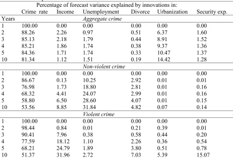
futher supported by the post sample VDCs as illustrated in Table 10. A substantial portion of

the variance of aggregate crime (88.26%) is explained by its own innovations in the short

run, for example, at two year horizon. In the long run, for example, at ten year horizon, the

portion of the variance of aggregate crime gradually decreases to 81.34% implying that other

variables explains about 19% of the shocks in the aggregate crime. The within sample VECM

results indicate nonviolent crime was Granger caused by unemployment. The post sample

VDCs further confirms this finding. Adding the relative strenght of income (8.85%) and

divorce rates (4.82%) to this impact, about 45.51% of the shocks in the nonviolent crime at

ten year horizon are accounted for the shocks in the unemployment, income and divorce rates.

(20)

However, a major portion (62.17%) of the variance in its forecast error at ten year horizon is

accounted for by the summation of five explanatory variables: income (31.96%),

unemployment (2.72%), divorce (7.03%), urbanization (5.39%), and security expenditures

[image:20.595.68.547.220.543.2]

(15.07%)

Table 10. Decomposition of Variance

Percentage of forecast variance explained by innovations in:

Crime rate Income Unemployment Divorce Urbanization Security exp.

Years Aggregate crime

1 100.00 0.00 0.00 0.00 0.00 0.00

2 88.26 2.26 0.97 0.51 6.37 1.60

3 85.13 2.18 1.79 0.44 8.91 1.52

4 85.21 1.86 1.74 0.38 9.37 1.36

5 84.36 1.71 1.74 0.33 10.47 1.37

10 81.34 1.12 1.51 0.19 14.42 1.28

'on)violent crime

1 100.00 0.00 0.00 0.00 0.00 0.00

2 86.67 0.13 10.25 2.92 0.01 0.01

3 76.98 1.73 18.80 2.81 0.01 0.16

4 68.32 4.41 24.07 2.99 0.01 0.16

5 58.80 6.50 28.60 4.07 0.01 0.15

10 53.56 8.85 31.84 4.82 0.07 0.14

Violent crime

1 100.00 0.00 0.00 0.00 0.00 0.00

2 98.44 0.84 0.01 0.21 0.39 0.01

3 90.41 7.96 0.38 0.58 0.44 0.20

4 77.59 18.12 1.10 2.26 0.36 0.54

5 68.21 24.79 1.89 3.80 0.51 0.78

10 51.37 31.96 2.72 7.03 5.39 15.07

Notes: Figures in the first column refer to horizons (i.e., number of years). All figures are rounded to two decimal places. The covariances matrices of errors from all the VECMs appeared to be very small and approaching zero suggesting that the combinations of all the variables in these models are linear. Therefore, the ortohogonal case for the variance decompositions are applied.

)%

This study has attempted to identify the causes of crime in Turkey using the cointegration

framework of Pesaran et al. (2001). The results indicate that the existence of cointegration

between crime categories, income, unemployment, divorce, urbanization and security

(21)

related to crime in a temporal causal relationship, in the long run, it is the dynamic interaction

of all these variables with each type of crime is causally related. In regards to long run partial

impacts of explanatory variables on crime categories, income seems to be main factor in

determining in all crime rates. This impact highest in total crime category but it is quite

similar in the case of violent and non violent crime. Unemployment is another major factor

contributor to all crime rates. However, in the case of violent crime, unemployment is

statistically insignificant. Divorce seems to be a positive effect in rising crime and that is

particularly high in the case of non violent crime. It is found that urbanization is contributing

to crime if they are in the category of violent offence. Although, the impact of security

expenditures appear to have deterring effect on crime but they are statistically not significant.

In within sample causality tests suggest that there is a long causality running from police

expenditures, urbanization, divorce, unemployment and income to all crimes. In the short run,

a bilateral causality between aggregate crime and income is detected. Similarly, a feedback

relationship is established between non violent crime and income. This finding of a long run

temporal relationship between all these variables is very important for the policy designers to

identify causation amongst the variables. Considering out of sample causalities, in the short

run, all crimes are mainly self feeding but as time horizon increases the causes of crime are

supported by income, unemployment and divorce rates. Security expenditures, however,

appears to deterring effect only in the case of violent crime in the long run. The results from

this analysis allow policy designers obtain additional insight as to what percentage of each

category of crime is explained by each determinant. As a passing note, it is plausible to

suggest that the overall results of this study could have been improved significantly if the

conviction rates were replaced by crime index.

The findings from this study present the dynamics of aggregate, violent and non violent crime

(22)

scenarios of economic and development, the estimated model elasticities enable the policy

(23)

+

Data definition and sources

Data are collected from three different sources, namely; Statistical Indicators of Turkish

Institute of Statistics (TSI), Main Economic Indicators (MEI) of OECD and World

Development Indicators (WDI) of World Bank.

c0, c1, c2, : are the convicts of total, non violent and violent crime offences per 100,000

people in logarithm, respectively. Non violent offences consist of property, burglary, motor

vehicle theft, fraud, corruption, etc. Violent crimes include homicide, assault, rape, and

kidnapping. Source: TSI.

y : is the per capita real income in Turkish lira based on 2000 prices in logarithm. Source:

WDI.

u : is the unemployment rate in logarithm. Source: MEI.

d : is the crude divorce rate per 1000 people in logarithm. Source: TSI.

r: is the urbanization rate in logarithm. The urbanization rate is the proportion of people living

in the cities. Source: WDI.

s: is the per capita real public security expenditures in Turkish lira based on 2000 prices in

logaritm. The public security expenditures contain police and gendarme forces in the cities

and country sides. Source: TSI.

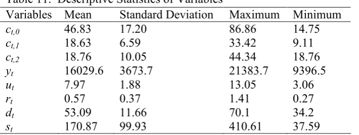
[image:23.595.124.479.618.752.2]

Descriptive statistics of the variables used in the econometric estimations are presented in Table 11.

Table 11. Descriptive Statistics of Variables

Variables Mean Standard Deviation Maximum Minimum

ct,0 46.83 17.20 86.86 14.75

ct,1 18.63 6.59 33.42 9.11

ct,2 18.76 10.05 44.34 18.76

yt 16029.6 3673.7 21383.7 9396.5

ut 7.97 1.88 13.05 3.06

rt 0.57 0.37 1.41 0.27

dt 53.09 11.66 70.1 34.2

(24)

*

Becker, G.S. (1968) Crime and punishment: an economic approach, Journal of Political Economy, ,-, 169 217.

Beki, C., Zeelenberg, K. and Kees, van M. (1999) An analysis of the crime rate in the Netherlands 1950 1993, British Journal of Criminology, ./, 401 415.

Bodman, P.M. and Maulty, C. (1997) Crime, punishment and deterence in Australia: a further empirical investigation, International Journal of Social Economics, 01, 884 901.

Britt, C. L. (1994) Crime and unemployment among youths in the United States, 1958 1990, American Journal of Economics and Sociology, 2., 99 109

Brown , K.V. (2001) The determinants of crime in South Africa, South African Journal of Economics, -/, 269 298.

Brown, R.L., Durbin, J., Evans, J.M. (1975) Techniques for testing the constancy of regression relations over time, Journal of the Royal Statistical Society, Series B, .,, 149 163.

Cantor, D. and Land, K.C. (1985) Unemployment and crime rates in the Post Wordl War II United States: a theoretical and empirical analysis, American Sociological Review, 23, 317 332.

Chiricos, T.G. (1987) Rates of crime and unemployment: an analysis of aggregate research evidence, Social Problems, .1, 187 212.

Corman, H. Joyce, T., and Lovitch, N. (1987) Crime, deterence and the business cyle in New York, The Review of Economics and Statistics, -/, 695 700.

Comertler, N. and Kar, M. (2007) Economic and social determinants of the crime rate in Turkey: cross section analysis, The Review of Faculty of Political Sciences of Ankara University, -0, 1 7.

Dickey, D. A. and Fuller, W. A. (1981) Likelihood ratio statistics for autoregressive time series with a unit root, Econometrica, 1/, 1057 1072.

Dickey, D. A. and Fuller, W. A. (1979) Distribution of the estimators for autoregressive time series with a unit root, Journal of American Statistician Association, 13, 12 26.

Detotto, C., and Pulina, M. (2009) Does more crime mean fewer jobs? An ARDL model, Working Papers, No.2009/5, Crenos, Cagliari, Italy.

Edmark, K. (2005) Unemployment and crime: is there a connection?, Scandinavian Journal of Economics, 43,, 353 373.

(25)

Ehrlich, I. (1973) Participation in illegitimate activities: a theoretical and empirical investigation, Journal of Political Economy, .5, 521 565.

Engle, R. F. and Granger, C. W. J. (1987) Cointegration and error correction: representation, estimation and testing, Econometrica, 22, 251 276.

Elliot, G., Rothenberg, T. and Stock, J. (1996) Efficient tests for an autoregressive unit root, Econometrica, -1, 813 836.

Funk, P., and Kugler, P. (2003) Identifying efficient crime combating policies by VAR models; the example of Switzerland, Contemporay Economics Policy, 04, 525 538.

Gartner, R. (1990) The victims of homicide: a temporal and cross national comparisons, American Sociological Review, 22, 92 106.

Hale, C. (1998) Crime and the business cycle in post Britain revisited, British Journal of Criminology, .5, 681 698.

Harrendorf, S., Heiskanen, M., and Malby, S. (2010) International Statistics on Crime and Justice, United Nations Office on Drugs and Crime, Vienna.

Johansen, S., and Juselius, K. (1990) Maksimum likelihood estimation and inference on cointegration with applications to money demand, Oxford Bulletin of Economics and Statistics, 20,169 210.

Kustepeli, Y., and Onel, G. (2006) Different categories of crimes and their socio economic determinants in Turkey: evidence from VECM, Conference Paper, presented at Turkish Economic Association on International Conference on Economics, September 11 13, 2006, Ankara.

Lee, D.Y., and Holoviak, S.J. (2006) Unemployment and crime : an empirical investigation, Applied Economics Letters, 4., 805 810.

Luiz, J.M. (2000) Temporal association, the dynamics of crime, and their economic determinants: a time series econometric model of South Africa, Social Indicators Research, 2., 33 61.

Levitt, S. (1999) The changing relationship between income and crime victimization, Federal Reserve Bank of 'ew York Policy Review, 2, 87 98.

Machin, S., and Meghir, C. (2004) Crime and economic incentives, The Journal of Human Resources, .1, 958 970.

Masih, A.M.M., and Masih, R. (1996) Temporal causality and the dynamics of different categories of crime and their socioeconomic determinants: evidence from Australia, Applied Economics, 05, 1093 1104.

(26)

Melick, M. D. (2003) The relationship between unemployment and crime, The Park Place Economist, 44, 29 36.

Narayan, P., and Smyth, R. (2004) Crime rates, male youth unemployment and real income in Australia: evidence from Granger causality tests, Applied Economics, .-, 2079 2095.

Narayan, P.K. (2005) The savings and investment nexus for China: evidence from cointegration tests, Applied Economics, .,, 1979 1990.

Nikolas, D., Alexandros, G. (2009) The effect of socio economic determinants on crime rates: an empirical research in the case of Greece with cointegration analysis, International Journal of Economic Sciences and Applied Research, 0, 51 64.

Pesaran, M. H., Shin, Y., and Smith, R. J. (2001) Bounds testing approaches to the analysis of level relationships, The Journal of Applied Econometrics, 4-, 289 326.

Phillips, P.C.B. and Perron, P. (1988) Testing for a unit root in time series regression, Biometrika, ,2, 335 346.

Sims, C. A. (1980) Macroeconomics and reality, Econometrica, 15, 1 48.

Saridakis, G. (2004) Violent crime in the United States of America: a time series analysis between 1960 2000, European Journal of Law and Economics, 45, 203 214.

Scorcu, A., and Cellini, R. (1998) Economic activity and crime in the long run: an empirical investigation on aggregate data from Italy, 1951 1994, International Review of Law and Economics, 45, 279 292.

Shoesmith, G.L. (2010) Four factors that explain both the rise and fall of US crime, 1970 2003, Applied Economics, 10, 2957 2973.

Soares, R. (2004) Development, crime and punishment: accounting for the international differences in crime rates, Journal of Development Economics, ,., 155 184.