Estimating the Need for Single Family
Rehabilitation
Marc T. Smith, Margaret S. Murray and William O’Dell
1Abstract.
Data availability has been an issue in tracking changes in the con-dition of housing at the neighborhood level. Census data are of limited use, and other methods are expensive, time-consuming, and subject to bias. This paper proposes a methodology that uses variables obtained from property assessor files to develop estimates of the condition of the housing stock. The property appraiser provides parcel level information on housing units. The measure developed, the ratio of market value to unit value new, can be used to estimate the quantity and degree of sub-standard housing in a community. This variable implicitly incorporates other variables thought to be important in the determination of housing condition including age, size, and tenure of the unit. This study is unique in that it establishes a single measure of housing quality, it is relatively simple to implement, and it relies on data that is easy to obtain.
1. Introduction
The use of indicators at the neighborhood level has been expanding as a means to identify neighborhoods for the targeting of resources, for advocacy, to document need for grant applications, to track changes over time, and to measure success in community development strategies. As such, indicators are important to community residents, local governments, and nonprofit or-ganizations as a reflection of neighborhood quality of life. A central compo-nent of neighborhood change indicators has been measures of housing mar-ket activity. These include housing sales prices and rents, homeownership rates, vacant units, abandoned properties, and mortgage loan activity.
Data availability has been an issue in the ongoing tracking of housing variables at the neighborhood level. The Census provides data for block groups and census tracks, but the data are only collected every 10 years. A further problem with Census data is that the geography may not fit
neighborhood boundaries. As a result, local developers of neighborhood in-dicators have made extensive use of property assessor files. This data source
Flor-provides parcel level information on housing units (and other land uses). A typical property assessor file will include, at a minimum, the taxable value and estimated market value of the property, sales price and date, square footage of building, year a home was built, address, tenure, and lot size. With this data, it is possible to aggregate to a defined neighborhood bound-ary and compile information on homeownership, appreciation in sales prices, number of transactions, and abandoned properties. The data are based on recorded transactions and can be updated annually, or more fre-quently in some cases.
One important indicator of the housing situation in a neighborhood that is generally not available from the parcel data is the condition of the housing stock. This variable is one of six success measures recommended in a recent Neighborhood Reinvestment Corporation publication (2001, page 8) as it reflects the level of improvements in a neighborhood and the appearance of the neighborhood. To measure housing condition, local governments and nonprofit organizations typically rely on windshield surveys or other pri-mary data collection. However, such surveys are expensive, time consuming, and subject to inconsistency resulting from the judgment of different survey-ors. The inconsistencies also limit the potential to compare across neighbor-hoods and cities.
To address these issues and provide a method that allows estimates of the number of units in an area that are substandard or in need of rehabilita-tion, this paper describes a methodology based on the use of parcel data. It provides a standard approach that could be used statewide or even nation-ally to the extent that data are available and consistent.
2
.
Literature Review
Importance of Housing Condition Measures
Housing affordability is generally thought to be the greatest housing problem in the United States today, and an extensive literature examines in-dicators of this need at the national level (see, for example, Bogdan and Can, 1997, Nelson, 1994, and U.S. Department of Housing and Urban Develop-ment, 1994, 1999). Housing condition is given less attention on the national level when measuring housing need, yet the work of many community de-velopment corporations and other nonprofit housing entities, as well as local government programs, focus on the rehabilitation of housing. In particular, major shares of federal Community Development Block Grant (CDBG) and Home Investment Partnerships Program (HOME) funds are devoted to hous-ing rehabilitation in many communities, and they contribute to the rehabili-tation of some 200,000 units annually (U.S. Department of Housing and Ur-ban Development, 2001). In an environment of limited resources, increased questioning of the value of local programs, and competing interests, there is a need for local government and nonprofit organizations to be able to target
resources to areas of greatest need as well as demonstrate the need for hous-ing rehabilitation programs.
The seeming lack of concern for housing condition in the national con-text is in part because the quality of the housing stock has improved dra-matically over the past 60 years by common measures. These measures in-clude the average size of units and the percent of units without kitchen facili-ties, complete plumbing, or heating. For example, in 1940 over 50 percent of housing units in the United States were lacking some or all plumbing; by 1991 that number had fallen to 2.5 percent (Kutty, 1999). Thus, the appear-ance is that condition is no longer a cause for significant national concern. Yet approximately $100 to $200 billion of rehabilitation is carried out in the United States each year, an amount that approaches that spent in new con-struction (U.S. Department of Housing and Urban Development, 2001). It is estimated that about 765,000 homeowners live in small properties that are severely inadequate, and an additional 1.6 million are in homes with moder-ate problems (Belsky, 2002).
The problem at the local level is that lacking complete plumbing, lacking heating facilities, or lacking kitchen facilities are the only variables that have been available in the Census since 1970 to provide an indicator of housing condition. These variables do not reflect the structural integrity of the unit or aspects of the unit subject to wear and tear. It is units whose structural, physical condition is deteriorated that require interventions in the form of rehabilitation programs or possibly their removal from the housing stock. Further, units that are in need of rehabilitation are generally concentrated in particular neighborhoods, so that the incidence in specific neighborhoods is considerably higher than the average for the metropolitan area or the nation. Yet these units are an important affordable housing resource, and their con-dition influences the quality of life in a neighborhood. Belsky (2002) points to the need to estimate rehabilitation needs in a community to aid in planning and to make the case for funding to local officials.
Providing evidence of the quality of the local housing stock as well as fa-cilitating local housing policy decisions requires better indicators of housing condition than those available through the Census. Without better indicators of housing condition, planners, program administrators, and nonprofit hous-ing organizations cannot adequately specify need numbers in their houshous-ing plans, measure progress in addressing needs, nor target and make estimates of the resources required for demolition and replacement. Estimates of the number of substandard housing units in a locality would facilitate policy, advocacy, resource allocation, and targeting decisions as well as provide in-formation to facilitate grant applications. On a more practical level, better estimates of substandard housing are necessary to facilitate the preparation by local governments of the required housing elements of comprehensive plans as well as federal Consolidated Plans. A common indicator that can be
applied across jurisdictions would also facilitate comparisons.
Nationally, 27 percent of the housing units in the U.S. and 39 percent in central cities, are over 50 years old, an age at which substantial rehabilitation is often needed (U.S. Department of Housing and Urban Development, 2001). Our focus is on Florida, specifically the Tampa Bay region. Florida has a younger housing stock than the national average. However, the aging of the Florida housing stock, particularly in slower growing and rural counties, has resulted in the condition of the housing stock becoming increasingly an issue of concern.2 Pinellas County, our county for analysis, has an older
housing stock than the Florida norm as it includes two cities, St. Petersburg and Clearwater, which were settled earlier than many other areas of the state.
Given that measuring housing condition at the local level is important and that there is not an inexpensive and consistent method currently avail-able to develop a set of condition measures for all jurisdictions in a state (or the nation), we sought to develop such an indicator. The approach we have taken in this analysis is to consider the possibility of using housing unit characteristics that are available from the county property appraisers data-base to develop proxies for housing condition. In this way, we could develop gross estimates of the need for rehabilitation or replacement in the locality. Variables that are anticipated to be important indicators of housing quality and that are available from the appraisers database include age of the unit, size of the unit, whether the unit is owner occupied, and the market value of the unit.
Data on Housing Condition
As stated earlier, the Census provides limited variables on housing con-dition. The American Housing Survey (AHS) provides more information, but this information is based on a survey, and the sample does not allow esti-mates at the jurisdiction level for Florida’s over 400 local jurisdictions. Thus, the AHS is useful at the national and metropolitan level to estimate housing condition but of limited use at the local level.3 Further, the expectation is that
housing condition is a greater problem in rural areas where the housing stock is older, but where AHS data are inadequate. Another approach is to undertake windshield or other surveys of condition, but they are expensive, time consuming, and may not allow cross-jurisdiction comparisons due to different definitions and standards used by surveyors in different communi-ties. In Florida, the county property appraisers provide an estimate of hous-ing condition as one of the data points in their data on properties in a county. These assessments are of limited usefulness because there is wide variation
2 See Shimberg Center for Affordable Housing (2003) for a discussion of the age of the housing
stock across Florida counties and the need for rehabilitation.
3 We will use data from the AHS to estimate a model at the metropolitan level that can then be
across counties in the percentage of units considered substandard, well greater than the expected difference in quality. In fact, some of the counties in which most of the housing stock has been built in the last twenty years are rated by the county appraiser as having the highest percentage of below av-erage housing units in the state.
There is limited literature on using secondary data sources to develop measures of housing condition4, and we have found little work at the scale of
small local communities as we are analyzing. Schneider and Zwick (1988, 1995) attempted to develop a measure of substandard housing in two Florida localities using county property appraiser data and testing the findings of that data with fieldwork (windshield surveys). They found a set of variables that were potential predictors of substandard housing, including age, size, and value of the unit. Koebel used tax assessor data to measure housing quality and created a “housing quality index” which was then compared to housing code violations in Louisville, Kentucky (Koebel 1989). Although the index showed promise as a tool for classifying poor quality housing, it mis-classified many units. This work was based on two earlier papers (Stegman and Sumka, 1976 and Sumka, 1977) that also demonstrated the use of tax as-sessor data in relation to housing quality.
The American Housing Survey develops a housing quality that is re-ferred to as ZADEQ5. This variable is based on multiple occurrences across a
number of individual variables that are measures of housing deficiencies, such as leaks, electrical breakdowns, or plumbing breakdowns. Using this variable as a measure of housing quality, Kutty (1999) uses data from seven metropolitan areas to estimate a model of the determinants of structural ade-quacy. She finds that age of the building is the most important physical at-tribute determining structural adequacy. Interestingly, this variable is sig-nificant yet her measure of age is a categorical variable with the oldest cate-gory being over 20 years old. Based on the former standards for calculating depreciation for tax purposes as well as comments from housing profession-als regarding wear and tear on homes, our expectation is that around 40 years old is when we would expect to begin to see declines in structural qual-ity. Other important factors in determining structural adequacy in Kutty’s model include unit type, tenure, income of the occupants, and vehicle own-ership. Kutty finds that disparities in structural adequacy exist across met-ropolitan areas, between central cities and suburbs, and across population groups. Kutty’s paper also reviews past work in developing a set of vari-ables to describe housing quality that recognizes the multidimensional qual-ity of housing.
4 There is a literature on impacts of neighborhood quality on housing values as well as literature
on property maintenance, depreciation, and property value or rent (see Springer and Waller, 1996, for a brief review of that literature).
Tenure (owner versus renter occupancy) has been explored as a variable in several papers including Gatzlaff, Green, and Ling (1998), Galster (1983) and Henderson and Ioannides (1983). The basic argument is that owner-occupants have a greater incentive to maintain their units than renters, and that relative maintenance effort would be reflected in appreciation rates and in housing condition. While Galster finds strong evidence of the relationship that owner-occupied housing is in better condition, Gatzlaff, Grreen, and Ling find only weak evidence. Both empirical papers explore only the single family housing stock.
The data set that we are using to develop local estimates of housing con-dition is county property appraiser data (further information on the data are available by request from the authors). This data set includes characteristics of the housing unit but not of the household occupying the unit. Our focus will be on single-family housing units because the appraiser data does not have information on units in a multifamily structure, only the structure itself. Consistent with Kutty’s (1999) variables, we have information on age of the unit and tenure.
One problem with Census type data is that it is based on the responses of occupants. Thus, data on the size of the unit and the value are often viewed as being inadequate because of the self-reporting and lack of knowledge about the unit and market. If true, this view may limit comparisons of Cen-sus data to property appraiser data on the unit. However, Kiel and Zabel (1999) report that on average owner-occupants of housing units overvalue their units by about five percent. They conclude that the use of owner esti-mates of value will result in reliable estiesti-mates of prices. Our approach will be to compare results from the AHS with results using the county property ap-praiser data. The Kiel and Zabel result indicates that we can use a value vari-able (estimated value of housing unit) across the two data sets. This compari-son enhances the applicability of AHS data to a local situation.
3.
Method and Data
The data for this analysis come from the American Housing Survey (AHS) 1998 AHS Tampa-St. Petersburg metropolitan sample, and the 1998 Florida State Tax Assessor records. The American Housing Survey collects separate data samples for 60 large metropolitan areas, including Miami-Ft. Lauderdale and Tampa-St. Petersburg in Florida. Data for each metropolitan area are collected once every four years or fifteen metropolitan areas are col-lected each year. In both the national and the metropolitan data samples, data are collected specifically on the same housing unit from period to pe-riod making it possible to track the same unit over time. Data are also gath-ered on the occupants of the unit but, since the focus of the AHS is the hous-ing unit those data may and do change over time.
Tax appraiser6 data are collected on every parcel of land in the state of
Florida. These data are compiled at the county level. The county files contain a number of variables for each parcel. Our focus is on single family housing units, and for these the data available7 include most recent and second most
recent sales price, just value, assessed value, year built, square footage of the unit, land value, size of the parcel, and whether the homestead exemption is claimed8. Note that there is no data on the households occupying a unit. The
inclusion of parcel identification numbers permits geographic information system mapping and allows for the examination of various spatial issues. Schneider and Zwick (1988, 1995) have used county property appraiser data in two Florida applications to test the use of this data in the identification of substandard housing. They developed a set of decision criteria to identify substandard units using the appraiser data, then used fieldwork to test the conclusions.
Method
This analysis is primarily descriptive. It attempts to link housing quality indicators found in the American Housing Survey with data gathered by the county tax assessor. Our goal is to provide local planners and neighborhood organizations with an easily derived estimate of the number of units of be-low standard housing quality in cities, counties, and neighborhoods. The AHS calculated variable that identifies housing quality, ZADEQ, is used to measure quality for units in the AHS sample. Because there are few severely inadequate housing units (less than 2.4 percent), the variable ZADEQ was reduced from three categories (adequate, inadequate, and severely inade-quate), to two categories (adequate and inadequate).
The county property appraiser data does not measure household charac-teristics that might contribute to the quality of a housing unit, such as house-hold size, age of househouse-holder, and income. The work of Schneider and Zwick suggests that housing unit characteristics that are available from the county property appraiser data and contribute to the quality of a unit include age, value, and square footage. These variables will be tested directly and indi-rectly. As became apparent from the data, age is a particularly important variable in determining housing condition. Why is age important? As hous-ing units age, and without reinvestment in the buildhous-ing, the value of the building gradually declines as a percentage of the total property value (in an area experiencing extreme problems, both housing value and land value may
6 In Florida, the tax assessor is identified as the tax appraiser.
7 Because of idiosyncrasies of the data collection process, not all of the data are available in all
counties. Further, the data we use is from reports that the county property appraisers file with the state for purposes of state oversight of the process. Additional data are available on master files maintained by the county appraiser.
8 The homestead exemption is available for owner occupied units and excludes $25,000 for the
decline). The concept of change used by real property appraisers suggests that at some point the building value declines as a result of depreciation to a point where it become desirable to tear the building down and construct a new structure. Age does not in itself result in a substandard unit, as evi-denced by the older homes in prime neighborhoods in many cities, but age combined with deferred maintenance and upkeep will result in declining housing quality.
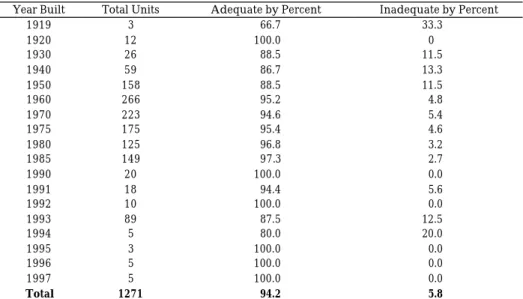
The method uses age, a variable that is available in both the AHS data-base and the tax appraiser data, as the starting point for the analysis. The AHS data indicate that there is a significant negative correlation between the age of the unit and its condition as evaluated by the variable ZADEQ. The calculated correlation coefficient is -.11 (.01). We then analyzed the relation-ship between specific age categories and the adequacy variable, ZADEQ. As seen in Table 1, the percentage of inadequate units generally increases with age. Figure 1 illustrates this relationship graphically. The methodology then attempts to build a relationship between the percentage of AHS units that are inadequate by age of unit and the characteristics of units of that age in the county property appraiser data set.
Table 1. Quality by Year Builta
Year Built Total Units Adequate by Percent Inadequate by Percent
1919 3 66.7 33.3 1920 12 100.0 0 1930 26 88.5 11.5 1940 59 86.7 13.3 1950 158 88.5 11.5 1960 266 95.2 4.8 1970 223 94.6 5.4 1975 175 95.4 4.6 1980 125 96.8 3.2 1985 149 97.3 2.7 1990 20 100.0 0.0 1991 18 94.4 5.6 1992 10 100.0 0.0 1993 89 87.5 12.5 1994 5 80.0 20.0 1995 3 100.0 0.0 1996 5 100.0 0.0 1997 5 100.0 0.0 Total 1271 94.2 5.8
a Note: Totals vary between tables due to missing data.
After examining the AHS data for the Tampa Bay area (Tampa and St. Petersburg), we then considered the tax assessor data from Pinellas County, Florida. Pinellas County is located on the west coast of Florida and contains the cities of St. Petersburg and Clearwater. The City of Tampa is adjacent but located in Hillsborough County. The analysis focuses on only single family housing because by doing so it is possible to evaluate just the housing unit and not the total property, as would be the case with multi-family property.
Although we recognize that significant condition problems are also present in multi-family housing, the property appraiser data did not permit the building value to be separated into unit values.
Figure 1. Percent of Inadequate Units by Age
In addition to age (year built), variables from the tax assessor data used in the analysis include just value9, land value, square footage, and latest sale
price. A number of new variables were then calculated. The variable land ratio is the ratio of land value to just value10.
Land ratio = Assessor estimate of land value / Assessor estimate of just value
The reciprocal of this variable was used to estimate the proportion of to-tal property value that is attributable to the building.
Percent of value attributed to building = 1 – Land ratio
9 Just value may or may not be the same as assessed value. In 1992, Florida passed the “Save Our
Homes” legislation. This legislation limits the annual increases in the assessed value of owner occupied (properties with homestead) houses to the lower of 3 percent of the assessed value of the property the prior year or the percent change in the CPI. The legislation became effective in 1994. For more information on the effects of this legislation see Gatzlaff. 1994.
10 This essentially the same as the land-to-value ratio calculated in real estate investment
analy-sis. 0 5 10 15 20 25 30 35 0 10 20 30 40 50 60 70 80 90 Age Percent Inadequate
Building value for each single-family unit was calculated two ways; first using the just value figure, and then using the latest sale price figure. Just value is the county property appraiser’s estimate of market value. However, if the latest sale price was recent and higher than the just value figure, it was used as a better indicator of market value.
Building value = (Percent of value attributed to the building)(Just value) or
Building value = (Percent of value attributed to the building)(Latest sale price)
Square footage of the unit enters the analysis indirectly as we also esti-mate the value of a new unit of that size as a way to approxiesti-mate the re-placement cost for the structure. To do this, we relied on the square foot es-timate of construction cost from the Marshall Valuation Service (1999) for the Southeast United States with an adjustment for the Tampa area. The average construction cost per square foot multiplied by the square foot figure for each unit produced the variable unit value new.
Unit value new = (Per square foot construction cost)(Square footage of unit)
Lastly, the ratio of current unit value to the replacement cost, the value ratio, was calculated.
Value ratio = Current unit value / Unit value new
This variable was then used to estimate the extent of investment in the unit since it was built. In other words, higher current unit values are indica-tive of units that have been maintained and upgraded over the years. Higher
Value Ratio numbers indicate units with values close to replacement cost.
That is, as this variable approaches one, the current value of the existing unit approaches the value of a new unit of the same size.
Because we wanted to evaluate differences between owner occupied and rental property, the tax appraiser data were divided into two groups. One group consisted of housing units claiming the homestead exemption11 and
the second group was made up of units where no exemption is claimed. This division may not correctly identify all owner occupied houses as some fami-lies may own two homes, one in Florida and one located elsewhere. Only the home that they reside in more than six months of the year and that they iden-tify as their principal residence qualifies for the homestead exemption.
11 Florida’s constitution provides for a $25,000 exemption, which is deducted from a property’s
assessed value if the owner qualifies. Applicants who timely file by March 1, possess title to the real property, and are bona fide Florida residents living in the dwelling and making it their permanent home as of January 1, qualify for the exemption. Properties granted Homestead Ex-emption also automatically receive the "Save Our Homes", Amendment 10, benefit.
Table 2 illustrates the mean and standard deviation of the variable, value
ratio, for both single-family, owner occupied and single-family rental units.
The mean value for owned units suggests that existing units are valued at about 71 percent of a new unit of equal size. Similarly, rental units are valued at about 65 percent of a new unit. A number of units have ratios above one. These are housing units that are valued at more than the cost to construct an average unit in the Tampa Bay area. Values above one can occur because the unit is of higher than average quality or because the unit has already been substantially upgraded and those upgrades represent above average quality. However, in the majority of cases as the unit deteriorates, the value of the ratio declines. At some point, rehabilitation becomes necessary in order to keep the unit livable. One question that we attempted to answer was: Where does that point occur? To answer that question, we compared tax assessor data with AHS data.
Table 2. Range of Value Ratios by Tenure
#Units Mean Deviation Standard
Owner Occupied 180,558 units .7087 .2194
Rental 42,554 units .6538 .2864
4. Results
The AHS data reports the year the building was built each year for the first ten years following construction (we refer to these as age groups 1 through 10), then age is reported in five-year increments for the next 20 years (age groups 11 through 14 cover these 20 years, units aged 11 through 30 years old). Lastly, ten-year periods are identified (these are our age groups 15 through 20, covering units aged 31 through 90 years old). In order to get an estimate of the age when significant problems begin to occur, the variable ZADEQ was cross-tabulated with AGE. Inadequate quality units began showing up around age group 11, units that were from 11 to 15 years old. As age increased, so did the incidence of inadequate quality12.
Turning then to the tax appraiser data, we began looking for the point at which the value ratio of units between 10 and 15 years of age began to fall into two groups, Adequate Quality and Needs Rehabilitation, in proportion to the relationship for units of that age as measured by the AHS data. In other words, did housing units fall into two quality groups of comparable
12 The analysis uses age groups identified in the AHS data. Collapsing data into ten-year
tion to the AHS distribution at age category 11 if the value ratio were sepa-rated into groups at say .9 or .8. Actually, at those high levels, housing units began to fall into the Needs Rehabilitation category at age four. The value
ratio was evaluated at successively lower levels until units became classified
into two groups at age group 11 (units 11 to 15 years old). This occurred when the value ratio was .45. At that point, the market value of the housing unit is only worth 45 percent of the value of new unit of average quality (re-placement cost). The relationship between the value ratio and the housing units falling into the needs rehabilitation category continued housing units in the succeeding age categories, categories 12 through 20 (units aged 16
through 90 years old). Note that the number of observations diminishes after 90 years.
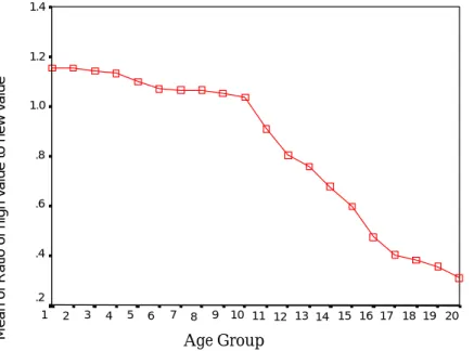
A one-way analysis of variance (ANOVA) was used to confirm the effect age has on housing quality as measured by the value ratio. This method fo-cuses on the differences between the means of the value ratio at each succes-sive age level testing the null hypothesis of no difference. The appropriate test statistic is the F ratio. There was a significant main effect. These results are presented in Table 3. Tukey’s post hoc test indicated groups 1 through 10 were all significantly different from age groups 11 through 20.
Figure 2. Means Plot – Owned Units Age Group 20 19 18 17 16 15 14 13 12 11 10 9 8 7 6 5 4 3 2 1 1.4 1.2 1.0 .8 .6 .4 .2
Figure 3. Means Plot – Rental Units
Table 3. One-Way ANOVA
Ratio of high value to new value – Owned Units
Sum of Squares df Mean Square F Sig. Between Groups 4848.447 19 255.181 11981.718 .000 Within Groups 3845.020 180538 2.130E-02
Total 8693.467 180557
Ratio of high value to new value – Rental Units
Sum of Squares df Mean Square F Sig. Between Groups 1541.590 19 81.136 1770.169 .000 Within Groups 1949.561 42534 4.584E-02
Total 3491.152 42553
Figure 2 and Figure 3 portray this relationship graphically. In both fig-ures the plot begins decreasing at an increasing rate around the 10 to 11 year age group. One additional fact that is seen when comparing the two figures is that the decline in quality begins earlier for rental units.
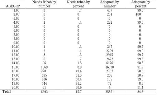
Following this, the value ratio was cross tabulated with age. The cross tabulations were calculated for owner occupied and rental units separately and are presented in Table 4a and 4b. In line with expectations that rental units would be more likely to need rehabilitation than owner occupied
Age Group 20 19 18 17 16 15 14 13 12 11 10 9 8 7 6 5 4 3 2 1
Mean of Ratio of high value to new value
1.4 1.2 1.0 .8 .6 .4 .2
units13, there is a marked difference between the percent of houses needing
rehabilitation, as reflected by the value ratio, in owned units versus rented units. Only 5.5 percent of the owned units are classed as needing rehabilita-tion while 15.7 percent of the rental units are.
Table 4a. Age Group and Quality: Owned Units
AGEGRP Needs Rehab by number Needs rehab by percent Adequate by number Adequate by percent
1.00 0 0 949 100.0 2.00 0 0 1280 100.0 3.00 0 0 1402 100.0 4.00 0 0 1405 100.0 5.00 0 0 1604 100.0 6.00 0 0 1687 100.0 7.00 0 0 1672 100.0 8.00 0 0 1430 100.0 9.00 0 0 1906 100.0 10.00 0 0 2140 100.0 11.00 5 .0 15513 100.0 12.00 11 .1 18690 99.9 13.00 17 .1 17715 99.9 14.00 246 .7 33339 99.3 15.00 3148 4.8 63075 95.2 16.00 4339 40.7 6314 59.3 17.00 890 73.9 314 26.1 18.00 683 82.9 141 17.1 19.00 546 87.2 80 12.8 20.00 16 94.1 1 5.9 Total 9901 5.5 170657 94.5
Table 4b. Age Group and Quality: Rental Units AGEGRP Needs Rehab by number Needs rehab by percent Adequate by number Adequate by percent 1.00 3 .7 457 99.3 2.00 0 0 261 100 3.00 0 0 0 0 4.00 1 .4 222 99.6 5.00 0 0 0 0 6.00 0 0 0 0 7.00 0 0 0 0 8.00 0 0 0 0 9.00 0 0 0 0 10.00 1 .3 347 99.7 11.00 2 .1 2209 99.9 12.00 8 .3 2945 99.7 13.00 6 .2 2672 99.8 14.00 96 1.5 6176 98.5 15.00 1569 8.9 16030 91.9 16.00 2701 49.4 2767 50.6 17.00 895 81.3 206 18.7 18.00 636 80.4 155 19.6 19.00 744 91.2 72 8.8 20.00 31 88.6 4 11.4 Total 6693 15.7 35861 84.3
13 See Gatzlaff, Green, and Ling.., and Galster for discussions of the maintenance of owners
5. Discussion
This research was motivated by a search for a simple yet accurate method by which housing quality could be estimated in a local jurisdiction. The current alternatives are to use Census data, which is limited in terms of the measures that can be employed as well as becoming out-of-date as the distance from the last Census lengthens, or to use housing surveys.
Tracking changes in housing quality is often compared to shooting at a moving target. After establishing the presence of a kitchen and plumbing as an indicator of adequate quality, the target moved. The complex model de-veloped by the AHS will not help local planners estimate local housing con-ditions. In this paper, we have presented a model based on the relationship between the adequacy of housing and the age of housing that emerges from AHS data. A measure, the ratio of market value to unit value new, derived from the county property appraiser data sets, is then used to test its correla-tion to the AHS relacorrela-tionship between condicorrela-tion and age. The relacorrela-tionship is such that we conclude that this single measure, value ratio, can be used to estimate the quantity and degree of substandard housing in a community. This variable implicitly incorporates other variables thought to be important in the determination of housing condition including age, size, and tenure of the unit. This study is unique in that it establishes a single measure of hous-ing quality, it is relatively simple to implement, and it relies on data that is easy to obtain. The methodology is based on the Tampa Bay area of Florida, and warrants testing in other areas in which the age and other characteristics of the housing stock differ.
References
Bogdan, Amy S. & Ayse Can. 1997. Indicators of local housing affordability: Comparative and spatial approaches. Real Estate Economics 25(1). 43-80. Galster, George C. Empirical evidence on cross-tenure differences in home
maintenance and conditions. Land Economics 59, 107-113.
Gatzlaff, Dean. 1994. An analysis of the recently enacted save our homes amendment: Its potential impact on the Florida real estate market. Flor-ida Real Estate Commission Education and Research Foundation. Talla-hassee, FL.
Gatzlaff, Dean H., Richard K. Green, & David C. Ling. 1998. Cross-tenure differences in home maintenance and appreciation. Land Economics 74, 328-342.
Henderson, J. V. & Y. M. Ioannides. 1983. A model of housing tenure choice.
American Economic Review 73, 98-113.
Website: http://www.ccappraiser.com/exemptn.htm - Homestead Exemp-tion. March 16, 2000.
Kiel, Katherine & William Zabel. 1999. The accuracy of owner-provided house values: The 1978-1991 American housing survey. Real Estate
Eco-nomics 27, 263-298.
Koebel, C. Theodore. 1986. Estimating substandard housing for planning purposes, Journal of Planning Education and Research 5, 191-202. Kutty, Nandinee. 1999. Determinants of the structural adequacy of
dwell-ings. Journal of Housing Research 10, 1.
Marshall & Swift. 1999. Residential cost handbook.
Nelson, Kathryn P. 1994. Whose shortage of affordable housing? Housing Policy Debate 5(4).
Schneider, Richard H. & Paul D. Zwick. 1988. Substandard housing in Alachua County: An inventory and identification methodology. Final report to the Alachua County Housing Authority, Gainesville, Florida Schneider, Richard H. & Paul D. Zwick. 1995. University of Florida – City of
Largo housing research project. Final report to the City of Largo, Flor-ida.
Shimberg Center for Affordable Housing, University of Florida. 2003. The
State of Florida’s Housing. Gainesville, Florida
Stegman, Michael A. & H. J. Sumka. 1976. Non-metropolitan Urban Housing:
An Economic Analysis of Problems and Policies. Cambridge, MA, Ballinger
Publishing Company.
Sumka, H. A. 1977. Measuring the quality of housing: an economic analysis of tax appraiser data. Land Economics 53, 198-309.
U.S. Department of Housing and Urban Development. 1994. Regional Housing
Opportunities for Lower Income Households. Washington, D.C.: Office of
Policy Development and Research.
U.S. Department of Housing and Urban Development. 1999. The Widening
Gap: New Findings on Housing Affordability in America. Washington, D.C.
U.S. Department of Housing and Urban Development. 2001. Barriers to the
Rehabilitation of Affordable Housing, Volume I: Findings and Analysis.
Wash-ington, D.C.
U.S. Department of Housing and Urban Development. Office of Policy De-velopment and Research. 2001. Recent Research Reports, December. Washington, D.C.