Munich Personal RePEc Archive
Stability of Demand for Money Function
in Nepal: A Cointegration and Error
Correction Modeling Approach
Bhatta, Siddha Raj
Tribhuvan University, Kathmandu Nepal
11 April 2011
Online at
https://mpra.ub.uni-muenchen.de/41404/
1
Stability of Demand for Money Function in Nepal: A Cointegration and Error Correction Modeling Approach
Siddha Raj Bhatta
Assistant Director at Nepal Rastra Bank, Kathmandu, Nepal
ABSTRACT
This paper examines the long run and short run demand for money functions and their stability issues for Nepal using the annual data set of 1975-2009 by using the recently developed ARDL modeling to cointegration popularized by Pesaran and Shin (1999). The bounds test shows that there exists the long run cointgrating relationship among demand for real money balances, real GDP and interest rate in case of both narrow and broad monetary aggregates. Further, the CUSUM and CUSUMSQ test reveal that both the long run narrow and broad money demand functions are stable. The results show that demand for real money balance in Nepal is a stable and predictable function of a few variables and the central bank can rely on the monetary aggregates as intermediate targets for achieving the broad economic objectives.
Keywords: money demand function, cointegration, error correction modeling
JEL Classification Code: E, E4, E41
1. INTRODUCTION
A good understanding of the determinants of the demand for real money balances in the economy by investigating the behavior of the money demand function is crucial for the formulation and implementation of an effective monetary policy. Moreover, the identification of a stable relationship between the demand for money and its determinants provides empirical evidence that the monetary targeting is an appropriate framework for economic stabilization policy (Rutayisire, 2010). That is, if the demand for real balances has a consistent or stable relationship with its determinants, the changes in money stock has predictable effects on income and output and the required change in the money stock to restore the equilibrium in the economy can be easily worked out. This is what needed for the stability of the economy. In such a case, the central bank can bring the desired changes in the economy by using monetary aggregate as a target variable. Thus, if the central bank relies on control of monetary aggregates as its policy instruments, it must believe in a known and reliable connection between changes in that aggregate and changes in the arguments of the money demand function in order for its policy to have predictable effects on those arguments. If instead the central bank relies on interest rates as targets and adjusts the monetary aggregate through daily reserve management to whatever level is required to hit them, instability of the demand for money could make the required reserve changes both large and unpredictable. In such a case, disorderly financial markets might well result (Cameron 1979).
For any central bank, stability issue of the money demand function is one of the most important guiding policy issues that helps decide whether to use the monetary targeting strategy or inflation targeting strategy in the monetary policy in bringing the desired changes in the economy. This issue has been triggered further by the abandonment of monetary targeting strategy by many developed countries such as Canada, Newzeland, Brazil, Turkey, Norway, Australia, etc as they switched to inflation targeting strategy arguing that the demand for money function has tending to become unstable due to financial liberalization. Stability of the demand for money function is, therefore, the focal point for any central bank‟s policy. In this context, an assessment of the monetary policy of Nepal requires first to test the stability of money demand function. The central bank of Nepal has been using money stock as the intermediate target of the monetary policy. Especially after the adoption of financial liberalization in the 1980s, as argued by Khan and Wadud (2003), there might have been the forces that might have caused the instability in money demand function and rendered the monetary policy ineffective. In such a case, the stability issue of the money demand function needs an intense focus for justifying the working of the monetary targeting strategy.
2
variable (interest rate) in Nepal and to examine the long run stability issue of the money demand function.
The rest of the paper is structured as follows. Section 2 presents the review of some studies at international and national level and justifies the need of the study, section 3 presents the methodology and discusses the data sources and section 4 synthesizes the estimation results and the last section presents the concluding remarks.
2. LITERATURE REVIEW
In literature, money demand function has been studied using many approaches. Goldfeld (1973), Boughton (1981), Arango and Nadiri (1981), Butter and Fase (1981), Mehra (1991), etc are a few among the vast pool of the authors who made a significant contribution in this field banking on the conventional models. The following section presents a review of the empirical studies on the money demand function at international level and national level.
2.1. Review of International Empirical Studies
In international context, different authors like Taylor, Lumas and Mehra, Hamori and Hamori, Bahmani-Oskooee, Chi Wing Ng, Halicioglu and Ugur, Akinlo, Ashsani, Omer, etc have examined the demand for money issue for different countries using cointegration analysis. A short review of the studies has been provided in the appendix A.
2.2. Review of National Empirical Studies
Empirical studies at the national level using the latest techniques of cointegration and error correction modeling are still lacking. The main problem behind this is lack of sufficient data observations, lack of high frequency data etc. A brief review of the studies in Nepalese context has been provided in appendix B.
The studies at international level imply that most of the studies in the money demand function in the international level have used cointegration analysis. It is because the results from OLS estimation can suffer from spurious regression phenomenon if the data are non-stationary. When the standard assumption of stationarity breaks down, straightforward application of regression technique no more remains valid. It therefore becomes necessary to look for the presence of unit roots, prevalence of cointegration and consequent application of error correction models (ECMs). Further, they give support to the use of ARDL modeling over other methods like Johansen multivariate cointegration technique, Phillips and Hansen technique, etc in case of annual data and/or small number of observation. It is because the validity of the result may be questioned in case of small size of sample in latter methods. They also reveal the fact that the real GDP, interest rate, inflation and exchange rate are the most common determinants of money demand. The national literature on the money demand function justifies the need of re-estimating the money demand function extending the data set beyond 1997 and examining the stability issue by using the suitable method valid for small sample. This study, thus, aims to overcome these shortcomings by extending the data set from 1975 to 2009 and by adopting the ARDL modeling to cointegration analysis proposed by Pesaran and Shin (1999) as a valid technique for small sample.
3. DATA AND METHODOLOGY 3.1. The General Model
In the literature of money demand function, the basic model of money demand begins with the following relationship:
M/P = f(S, OC)
Where, the demand for real balances M/P is a function of the chosen scale variable(s) to represent the economic activity and the opportunity cost of holding money (OC). M stands for the selected monetary aggregates in nominal term and P for the price (Sriram, 2000).
3.2. Selection of Variables Scale Variable
3
and Meltzer(1964), Chow(1966), Laidler (1966), Khan (1974), etc] while there are some emphasizing the use of wealth as a scale variable [Meltzer(1963), Hamberger (1966),etc] and some have used the measured income [Goldfeld (1973), Arango and Nadiri (1981), etc]. However, in the context of developing countries, measured income has been used in most empirical studies. Several studies in India [Gujarati (1968), Bhattacharya (1974), Sampath & Husain (1981), etc] have used current income as the scale variable. The reason for this may be two-fold: first, the information on wealth is not available in the non-monetized economy and secondly, permanent income series cannot be meaningfully constructed because of very short time series national income data. In the context of Nepal, several studies [Poudel (1989), Khatiwada (1997), Pandey (1998), Gaudel (2003)] have used real GDP as the scale variable and found significant and stable relationship between real GDP and the stock of money holding. Thus, following the literature, this study has selected real GDP as the scale variable.
Opportunity Cost Variable
Selection of opportunity cost variable also is not free of debate. There is the ongoing controversy as which interest rate is the best indicator of the opportunity cost of holding money. Some argue that the long-term bond rate is better choice as it is more representative of the average rate of return on capital. The Keynesian theory also supports the long term interest rate as it is the interest rate that is linked with investment decision and hence the level of income. Since the economic theory on the money demand function does not provide any clear cut guideline on the choice of interest rate, researchers have tried different interest rates in modeling the money demand function.
In case of US, Khan (1974) and Jacobs (1974) have used the long term rate of interest whereas Heller (1965) and Laidler (1971) have used short term interest rate. In case of India, Gupta (1970) and Bhattacharya (1974) have used the short term interest rate in the money demand function. In the context of Nepal, the use of T-bill rate or long term bond rate is irrelevant as these instruments are not a significant part of asset portfolios. Further, data are not available for long term fixed deposit rate for the whole study period. Thus, in this study, rate of interest on saving deposit has been used as a proxy to interest rate on short term financial assets to model the narrow money demand and the interest rate on one-year fixed deposit has been used as a proxy for long term interest rate to model the broad money demand function.
3.3 The Empirical Model
In this study, following Bahmani-Oskooee (2001), the following model has been considered.
ln𝑚𝑡 =𝑎+𝑏𝑙𝑛𝑦𝑡+𝑐𝑟𝑡+𝑒𝑡… … … …. (1)
Where, mt is a monetary aggregate in real term, y the real GDP, r the interest rate and e is a white noise error term. Based on the conventional economic theory, the income elasticity parameter, b, is expected to be positive whereas the interest elasticity parameter, r, is expected to be negative.
To model the money demand functions for both narrow and broad money aggregates, equation (1) can be written in the form of two different models: Model I for Narrow Money Demand Function and Model II for Broad Money Demand Function.
Model I Narrow Money Aggregate : ln𝑚1𝑡=a+b ln 𝑦𝑡+c𝑟𝑠𝑑𝑡+et……….(2)
Model II Broad Money Aggregate : ln𝑚2𝑡=a+b ln 𝑦𝑡+c𝑟𝑓𝑑𝑡+et……….(3)
The details of all the variables used in the formulation of equations (2), (3) and other variables used in this study have been presented in Table 1.
Table 1: Variable Details
Variables Name
Details
m1t Real Narrow Money Stock defined by the narrow money stock divided by CPI(FY
4
m2t Real Broad money stock defined by the broad money stock divided by CPI( FY
2000/01=100)
yt Real GDP defined by nominal GDP deflated by the implicit GDP deflator(FY
2000/01=100)
ln m1t Natural logarithm of real narrow money stock
ln m2t Natural logarithm of real broad money stock
ln yt Natural logarithm of real GDP
rsdt Rate of interest on saving deposit
rfdt Rate of interest on one-year fixed deposit
Narrow Money stock(M1)
Currency held by public plus demand deposits of the commercial banks (CC+DD)
Broad Money stock(M2)
Narrow money stock plus time deposits(CC+DD+TD)
CPI Consumer price index (FY 2000/01=100)
INF Expected rate of inflation proxied by the actual rate of inflation defined by ( CPIt -CPIt-1
)/CPIt-1
rrsdt Real rate of interest on saving deposit defined as nominal interest rate on saving
deposit minus expected rate of inflation
rrfdt Real rate of interest on 12-months fixed deposit defined as nominal interest rate on
such deposit minus expected rate of inflation
3.4. Estimation Methodology
There are various techniques for conducting the cointegration analysis on money demand function. The popular approaches are: the well-known residual-based approach proposed by Engle and Granger (1987) and the maximum likelihood approach proposed by Johansen and Julius (1990) and Johansen (1988). When there are more than two I(1) variables in the system, the maximum likelihood approach of Johansen and Julius has the advantage over residual-based approach of Engle and Granger; however, both of the approaches require that the variables have the same order of integration. This requirement often causes difficulty to the researchers when the system contains the variables with different orders of integration. To overcome this problem, Pesaran et al. (1996, 2001) proposed a new approach known as Autoregressive Distributed Lag modeling (ARDL) to cointegration which does not require the classification of variables into I(0) or I(1). It has numerous advantages in comparison to other cointegration methods such as Engle and Granger (1987), Johansen (1988), and Johansen and Julius (1990) procedures: (i) it can be applied on a time series data irrespective of whether the variables are I(0) or I(1) (Pesaran and Pesaran, 1997)), while Johansen cointegration techniques require that all the variables in the system be of equal order of integration, (ii) it takes sufficient numbers of lags to capture the data generating process in a general-to-specific modeling framework (Laurenceson and Chai, 2003). (iii) while the Johansen cointegration techniques require large data samples for validity, the ARDL procedure is statistically more significant approach to determine the cointegration relation in small samples, (iv) A dynamic Error Correction Model (ECM) can be derived from ARDL through a simple linear transformation (Banerjee et.al., 1993). The ECM integrates the short-run dynamics with the long run equilibrium without losing long-run information. (v) The ARDL procedure allows that the variables may have different optimal lags, while it is impossible with conventional cointegration procedures, (vi) The ARDL technique generally provides unbiased estimates of the long-run model and validates the t-statistics even when some of the regressors are endogenous, (vii) The ARDL procedure employs only a single reduced form equation, while the conventional cointegration procedures estimate the long-run relationships within a context of system of equations.
Following the ARDL approach proposed by Pesaran and Shin (1999), the existence of long run relationship could be tested using equation (4) below:
∆ln 𝑚𝑡=𝑎0+ 𝑏𝑗∆ln𝑚𝑡−𝑗 𝑝
𝑗=1
+ 𝑐𝑗∆ln𝑦𝑡−𝑗 𝑞
𝑗=0
+ 𝑑𝑗∆𝑟𝑡−𝑗+𝛾1ln𝑚𝑡−1 +𝛾2ln𝑦𝑡−1 +𝛾3ln𝑟𝑡−1+𝜉𝑡
𝑟
𝑗=0
5
Where, mt represents real narrow money balances for narrow money demand model (model I) and real broad money balances for broad money demand model(model II), r represents interest rate on saving deposit for model I and interest rate on one-year fixed deposit for model II. Similarly, γ1 ,γ2
and γ3 are the long run coefficients while, bj,cj, dj and ζt represents the short run dynamics and random disturbance term respectively.
3.5. Hypothesis
To test whether the long run equilibrium relationship exists between demand for real money balances, real GDP and interest rate, Bounds test (F-version) for cointegration is carried out as proposed by Pesaran and Shin (1999). To test the long run level relationship between the variables, the hypotheses are:
Null Hypothesis: 1 =2 =3 =0 i.e. the long run relationship does not exist.
Alternative hypothesis: 1 ≠ 2 ≠ 3 ≠ 0 i.e. the long run relationship exists.
This hypothesis is tested by means of the familiar F statistic. The distribution of this F-statistics is non-standard irrespective of whether the variables in the system are I(0) or I(1). The critical values of the F-statistics in this test are available in Pesaran and Pesaran (1997) and Pesaran et al. (2001). They provide two sets of critical values in which one set is computed with the assumption that all the variables in the ARDL model are I(1), and another with the assumption that they are I(0). For each application, the two sets provide the bands covering all the possible classifications of the variables into I(0) or I(1), or even fractionally integrated ones. If the computed F-statistics is higher than the appropriate upper bound of the critical value, the null hypothesis of no cointegration is rejected; if it is below the appropriate lower bound, the null hypothesis cannot be rejected, and if it lies within the lower and upper bounds, the result is inconclusive (Samreth, 2008).
Next step is the estimation of the long run relationship based on the appropriate lag selection criterion such as adjusted R2, Schwarz Bayesian Criterion (SBC), Akaike Information Criterion (AIC) and Haann Quinn (HQ) Criterion. Based on the long run coefficients, the estimation of dynamic error correction will be carried out using formulation of equation (5). The coefficients δ1i, δ2i, andδ3i show the short run dynamics of the model and δ4 indicates the divergence/convergence towards the long run equilibrium. A positive coefficient indicates a divergence, while a negative coefficient indicates convergence. The term ECM is derived as the error term from the corresponding long run model whose coefficients are obtained by normalizing the equation on m1t and m2t respectively for both money demand models.
∆ln 𝑚𝑡=𝛿0+ 𝛿1𝑗∆ln𝑚𝑡−𝑗 𝑝
𝑗=1
+ 𝛿2𝑗∆ln𝑦𝑡−𝑗 𝑞
𝑗=0
+ 𝛿3𝑗∆𝑟𝑡−𝑗+𝛿4𝐸𝐶𝑀𝑡−1
𝑟
𝑗=0
+𝜐𝑡…(5)
For the test of stability, CUSUM and CUSUMSQ tests as proposed by the Brown et al. (1975) have been carried out. Besides these tests, a battery of other tests are also carried out, such as Lagrange Multiplier (LM) test for serial correlation, Ramsey Reset test for functional form Misspecification, Jarque-Berra Test for normality and KB test for heteroscedasticity.
3.9. The Data
This study is based on the secondary data. The data sources are Quarterly Economic Bulletin published by Nepal Rastra Bank (NRB), Economic Survey published by Ministry of Finance (MOF) and the World Economic Outlook by IMF. The GDP figures have been extracted from the World Economic Outlook database of IMF available at econstats.com ( FY 2000/01 base year). The information pertaining to the money balances and interest rates on saving and one-year fixed deposit have been extracted from Quarterly Economic Bulletin (various issues). The data on the CPI (FY 2000/01=100) have been extracted from the Economic Survey 2009/10.
4. Estimation Results
6
cannot be used. With the ADF test, is has been confirmed that none variables are integrated of order higher than one.
Following the Auto Regressive Distributed Lag Modeling (ARDL) to the formulation of money demand function as popularized by Pesaran and Shin (1997), the bounds test (F-statistics) has been applied to justify the existence of the cointegration or long-run relationship among variables in the system. Table 2 provides the results of the F-statistics according to various lag orders.
Table 2: F-statistics (Bound Test)
Lag order 0 1
F statistic M1 Aggregate 3.75 4.55* M2 Aggregate 7.65** 4.94**
Note: The relevant critical value bounds are (with intercept and no trend; number of regressors = 2) 3.79 – 4.85 at the 95% significance level and 3.18– 4.12 at the 90% significance level; * denotes that the F-statistic falls above the 90% upper bound and ** denotes above the 95% upper bound.
The results of Table 2 shows that most of the F-statistics are above the upper bounds of the critical values (CV) of standard significance levels (5 % or 10%) provided by Pesaran and Pesaran (1997). But these critical values were generated on the basis of 40,000 replications of a stochastic simulation for a sample of 1,000 observations. So, they are less relevant for a small sample size. Therefore, following the critical values by Narayan and Smyth (2004) which are based on 40,000 replication of a stochastic simulation for a sample of 40 observations with two regressors, the critical value bounds are 2.83 to 3.58 at 10 % and 3.43 to 4.26 for 5% level of significance. On the basis of these critical values, the calculated F-statistics clearly rejects null hypothesis of no cointegration at 5 % or 10% level of significance. However, Bahmani-Oskooee and Rehman(2005) consider these results as preliminary, precisely due to arbitrary choice of lag selection, and rely more on the other stages of estimation for testing cointegration which are more efficient.
In the second step, equation (4) is estimated and different model selection criteria are used to justify the lag orders of each variable in the system. Only an appropriate lag selection criterion will be able to identify the true dynamics of the model. The maximum lag order is set to 2 following Pesaran and Shin (1999) and Narayan and Smyth (2004) as the data are annual and there are only 35 observations. With this maximum lag order, the adjusted sample period for analysis becomes 1977 to 2009. This setting also helps save the degree of freedom, as our available sample period for analysis is quite small. Using Microfit 5.0, all the selection criteria have given the same results. Microfit runs the (p+1)k numbers of regressions and selects the best model on the basis of different model selection criteria, where p is the maximum number of lags to be used and k is the number of variables in the equation. Here, the number of regressions to be run are (2+1)3 = 27. The ARDL (1, 0, 0) model is selected on the basis of all criteria like Adjusted R2, Schwarz Bayesian Criterion (SBC), Akaike Information Criterion (AIC) and Haann Quinn criterion for both M1 aggregate and M2 aggregate models. According to Pesaran and Pesaran (1997), AIC and SBC perform relatively well in small samples, although the SBC is slightly superior to the AIC (Pesaran and Shin, 1999). Besides, SBC is parsimonious as it uses minimum acceptable lag while selecting the lag length and avoid unnecessary loss of degrees of freedom. Therefore, SBC criterion has been used, as a criterion for the optimal lag selection, in all cointegration estimations.
After selecting the appropriate lag orders for each variable in the system, equation (4) is re-estimated. The results of such estimation along with the short run diagnostic statistics are presented in Table 3.
Table 3: Full-information ARDL Estimate Results (M1 monetary aggregate)
Autoregressive Distributed Lag Estimates
ARDL (1,0,0) selected based on Schwarz Bayesian Criterion Dependent variable is ln m1t
33 observations used for estimation from 1977 to 2009 Regressors
𝛥 ln m1t(-1)
𝛥 yt
𝛥 rsdt
C
Coefficient 0.51* 0.67* -0.002 -5.26*
7
R-Squared 0.99 R-Bar-Squared 0.99
S.E. of Regression 0.04 F-Stat. F(3,29) 1855.9[0.00] Diagnostic Tests
Test Statistics LM Version F Version A:Serial Correlation CHSQ(1) =0.33[0.56] F(1,28)= 0.28[0.59] B:Functional Form CHSQ(1) =3.87[0.04] F(1,28) = 3.72[0.06] C:Normality CHSQ(2) = 1.20[0.54] Not applicable D:Heteroscedasticity CHSQ(1) = 0.008[0.93] F(1,31) =.007[0.93]
Note: A: Lagrange multiplier test of residual serial correlation; B: Ramsey‟s RESET test using the square of the fitted values; C: Based on a test of skewness and kurtosis of residuals; D: Based on the regression of squared residuals on squared fitted values; *denotes the significance of coefficient at 5% level
Table 3 indicates that the overall goodness of fit of the estimated ARDL regression model is very high with the result of adjusted R2 = 0.99. From the diagnostic tests, it is clear that the model passes all of the tests. The critical values of 𝝌2 for one and two degrees of freedom at 5% level of significance are 3.84 and 5.99 respectively. Thus, null hypothesis of normality of residuals, null hypothesis of no first order serial correlation and null hypothesis of no heteroscedasticity are accepted. However, the null hypothesis of no misspecification of functional form can be accepted at 1% level of significance. The estimated long-run model of the corresponding ARDL (1, 0, 0) for the demand for narrow money balances is:
ln𝑚1𝑡 =−10.89 + 1.39 ln𝑦𝑡−0.0039𝑟𝑠𝑑𝑡
The long run coefficients are the values of coefficients 𝛾1 to 𝛾3 of equation (4) normalized on ln m1t by dividing the coefficients by the coefficient (-𝛾1).
[image:8.595.66.531.72.187.2]The long run coefficients are reported in Table 4. As expected, the coefficient of the real income (GDP) is positive and that of short term interest rate is negative. Quantitatively, the income elasticity of narrow money demand is 1.39, which is highly significant as reflected by a t-statistic of 27.40. This in turn shows that one percentage increase in real GDP leads to increase in the real money balance holdings by 1.39 percentages. Thus, money seems to be a luxury asset in Nepal. This result is in conformity with many studies done in underdeveloped countries e.g. Poudel (1989) and Khatiwada (1997) for Nepal, Aghevli et.al. (1979) and Teseng and Corker (1991) for Asian countries and Simmons (1992) for African Countries. It thus rejects the conclusion of Gaudel (2003) that income elasticity of demand for money is less than unitary in Nepal. The more than unity elasticity implies that an increase in income leads to a higher increase in the demand for real money balances and a reduction in the velocity of money (Rutayisire, 2010). This result is attributed to the under-monetization of the economy where the gradual absorption of the non-monetary sector by the monetary sector is accompanied by an increase in cash in hand that is faster than income.
Table 4: Estimated Long Run Coefficients using the ARDL Approach
ARDL (1,0,0) selected based on Schwarz Bayesian Criterion Dependent variable is ln m1t
33 observations used for estimation from 1977 to 2009 Regressors
ln yt
rsdt
C
Coefficient 1.39* -0.0039 -10.89*
T-Ratio[Prob] 27.40[0.00] -0.26 [0.79] -17.95[0.00]
*shows the significance of coefficients at 1% level of significance
8
individual out of his remuneration, investing the rest in assets and thereby reducing the interest elasticity of money demand to less than unity or even zero. The result that inflation also is not a significant opportunity cost of holding narrow money balances is in conformity with Pandey (1998) but in contradiction with several other studies done in developed countries. This result points to two possibilities: either the actual rate of inflation is not a good proxy of the expected rate of inflation or inflation does not have a significant impact upon the demand for real money balances in Nepal.
The estimates of the error correction representation of the ARDL (1, 0, 0) model selected by the SBC criterion are presented in Table 5. The long run coefficients are used to generate the error correction term .i.e. ecm = ln m1t-1.39 ln yt + 0.0039rsdt+10.89. The computed F-statistic clearly rejects the null hypothesis that all regressors have zero coefficients. The JB test for normality shows that the residuals of the error correction modeling are normally distributed. The KB test supports the homoscedasticity assumption. Importantly, the error correction coefficient has the expected negative sign and is highly significant as shown by the probability value being zero. This helps to reinforce the existence of cointegration as provided by the F-test. Specifically, the estimated value of ecm(−1) is
-0.482. The absolute value of the coefficient of ecm(−1) is substantially high indicating the fast speed
of adjustment to equilibrium following short-run shocks; about 48% of the disequilibrium, caused by previous period shocks, converges back to the long-run equilibrium in one period. The short-run coefficients show the dynamic adjustment of these variables. The coefficient of income and interest rate give the short- run elasticities of income and interest rate respectively. The short run income elasticity thus is 0.67 which is less than the long run elasticity 1.39. On the other hand, as in the long run, the short run elasticity of interest rate is not statistically significant implying that demand for money even in the short run remains independent of the interest rate. The adjusted R-square of the error correction model is rather low but it does not significantly affect our results since the variables are in the difference form. [For example see Omer (2010), Samreth (2008), Bahmani-Oskooee and Chi Wing Ng (2002)]. The low adjusted R square is due to the selection of a restricted error correction model without a constant term following Pesaran and Shin (1999).
Table 5: Error Correction Representation for the Selected ARDL Model
ARDL(1,0,0) selected based on Schwarz Bayesian Criterion Dependent variable is 𝛥ln m1t
33 observations used for estimation from 1977 to 2009 Regressors
𝛥ln yt
𝛥 rsdt
ecm(-1)
Coefficient 0.67* -0.0019 -0.48*
Standard Error 0.16
0.007 0.12
T-Ratio[Prob] 4.10[0.00] -0.26[0.79] -4.14[0.00]
R-Squared 0.37 R-Bar-Squared 0.30 S.E. of Regression 0.04 F-Stat. F(3,29) 5.73[0.003] JB(Normality) 1.20[0.54]
F-stat. (For KB heteroscedasticity test) : 0.09[0.75] ecm = ln m1t -1.39*ln yt + 0.0039*rsdt + 10.89*C
Note: R-Squared and R-Bar-Squared measures refer to the dependent variable 𝛥M1t and in cases where the error correction model is highly restricted, these measures could become negative; *shows the significance of coefficients at 1% level of significance.
Next, equation (4) is estimated for M2 monetary aggregates. Table 6 presents the estimated coefficients along with the diagnostic test statistics. The results are similar to the case of narrow money demand.
Table 6: Full-information ARDL Estimate Results (M2 Monetary Aggregate)
ARDL(1,0,0) selected based on Schwarz Bayesian Criterion Dependent variable is ln m2t
33 observations used for estimation from 1977 to 2009 Regressors
𝛥ln m2t(-1)
𝛥ln yt
𝛥rfdt
C
Coefficient 0.59* 0.72* -0.6579E-3 -5.70*
Standard Error 0.08
0.16 0.004 1.3
T-Ratio[Prob] 6.82[0.00] 4.42[0.00] -0.13[0.89] -4.26[0.00]
9
Test Statistics LM Version F Version A:Serial Correlation CHSQ(1) = 0.06[0.79] F(1,28) =0.05[0.81] B:Functional Form CHSQ(1) = 1.51[0.21] F(1,28) =1.34[0.25] C:Normality CHSQ(2) = 0.64[0.72] Not applicable D:Heteroscedasticity CHSQ(1) = 0.003[0.95] F(1,31) = .003[0.95]
Note: A:Lagrange multiplier test of residual serial correlation; B:Ramsey's RESET test using the square of the fitted values; C:Based on a test of skewness and kurtosis of residuals; D:Based on the regression of squared residuals on squared fitted values; *shows the significance of coefficients at 1% level of significance
From the diagnostic tests in table 6, it is clear that null hypothesis of no first order serial correlation and null hypothesis of no heteroscedasticity and null hypothesis of no misspecification of functional form can be easily accepted at 5% level of significance. The estimated long run money demand function for broad money aggregate is:
ln𝑚2𝑡 =−14.25 + 1.81 ln𝑦𝑡−0.0016𝑟𝑓𝑑𝑡 The long run coefficients are reported in Table 7.
Table 7: Estimated Long Run Coefficients using the ARDL Approach
ARDL(1,0,0) selected based on Schwarz Bayesian Criterion Dependent variable is ln m2t
33 observations used for estimation from 1977 to 2009 Regressors
ln yt
rfdt
C
Coefficient 1.81* -0.0016 -14.25*
Standard Error 0.07
0.01 0.90
T-Ratio[Prob] 23.48[0.00] -0.13 [0.89] -15.70[0.00]
Note: Figures in parentheses are the probabilities associated with the t-ratios and the asterisk * shows that the coefficient is significant at 1% level of significance.
As in the narrow money demand model, the coefficient of the real income (GDP) is positive and that of one year fixed deposit interest rate is negative. Quantitatively, the income elasticity of broad money demand is 1.81, which is highly significant as reflected by a t-statistic of 23.48. This in turn shows that one percentage increase in real GDP leads to increase in the real money balance holdings by 1.81 percentages. It also implies that the income elasticity for broad definition of money is higher than narrow money. This result is again in conformity with Poudel (1989) and Khatiwada (1997) for Nepal. The interest rate despite bearing the correct negative sign is again statistically insignificant which implies that in the long run, either, the demand for broad money balances remains independent of the interest rate or the chosen interest rate rfdt is not an appropriate opportunity cost variable. Here also, in search for an appropriate opportunity cost variable, the real rate of interest was tried but the coefficient of interest rate did not appear to be significant. This again is in conformity with the view of Johnson (1963). Finally, the rate of inflation also did not prove fruitful. As the intercept term is statistically significant, it implies that unidentified variables including time trend have significant bearings on real money demand and they have a negative impact on real money demand (Khatiwada, 1997).
The error correction representation for broad money aggregate model has been presented in table 8 which reconfirms the cointegrating relationship between the variables included in the broad money demand function as revealed by the expected negative sign with the error correction term with a highly significant probability value of zero. The long run coefficients are used to generate the error correction term .i.e. ecm = ln m2t- 1.81*ln yt + 0.0016*rfdt + 14.25*C. The computed F-statistic clearly rejects the null hypothesis that all regressors have zero coefficients. Specifically, the estimated value of ecm (−1) is -0.40. The absolute value of the coefficient of ecm (-1) is substantially high indicating the fast speed of adjustment to equilibrium following short-run shocks; about 40% of the disequilibrium, caused by previous period shocks, converges back to the long-run equilibrium in one period. Since, the absolute value of the coefficient of ecm is lower in case of broad money demand, there is a slower speed of adjustment of short run disequilibrium to the long run equilibrium in case of broad money demand function.
Table 8: Error Correction Representation for the Selected ARDL Model
ARDL(1,0,0) selected based on Schwarz Bayesian Criterion Dependent variable is 𝛥ln m2t
10
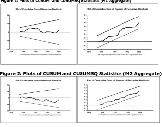
Figure 1: Plots of CUSUM and CUSUMSQ Statistics (M1 Aggregate)
Regressors Coefficient Standard Error T-Ratio[Prob]
𝛥ln yt 0.72 0.16 4.42[0.00]
𝛥rfdt -0.6579E-3 0.004 -0.13[0.89]
ecm(-1) -0.40 0.08 -4.55[0.00] R-Squared 0.41 R-Bar-Squared 0.35 S.E. of Regression 0.03 F-Stat. F(3,29) 6.98[0.00] ecm = ln m2t - 1.81*ln yt + 0.0016*rfdt + 14.25*C
JB(Normality) 0.64[0.72]
F-stat. (For KB heteroscedasticity test): 0.02[0.87]
Note: R-Squared and R-Bar-Squared measures refer to the dependent variable 𝛥M1 and in cases where the error correction model is highly restricted, these measures could become negative
The coefficient showing the short run dynamics are not all significant. Only the short run income elasticity (0.72) is significant where as the short run interest rate elasticity is not significant though having a correct sign implying that money demand in the short run also remains independent of the interest rate. All these coefficients show the dynamic adjustment of these variables.
Stability Test
[image:11.595.72.405.486.747.2]Finally, the stability of the long run coefficients together with the short run dynamics is examined. In doing so, Pesaran and Pesaran (1997) have been followed and the CUSUM and CUSUMSQ tests [proposed by Brown, Durbin, and Evans (1975) have been applied. The tests are applied to the residuals of the two models following Pesaran and Pesaran (1997). Specifically, the CUSUM test makes use of the cumulative sum of recursive residuals based on the first set of n observations and is updated recursively and plotted against break points. If the plot of CUSUM statistics stays within the critical bounds of 5% significance level represented by a pair of straight lines drawn at the 5% level of significance whose equations are given in Brown, Durbin, and Evans (1975)], the null hypothesis that all coefficients in the error correction model are stable cannot be rejected. If either of the lines is crossed, the null hypothesis of coefficient constancy can be rejected at the 5% level of significance. A similar procedure is used to carry out the CUSUMSQ test, which is based on the squared recursive residuals. Fig. 1 and fig. 2 show the graphical representation of the CUSUM and CUSUMSQ plots applied to the money demand models selected by the SBC criterion. Neither CUSUM nor CUSUMSQ plots cross the critical bounds, indicating no evidence of any significant structural instability. Similar results have been obtained for the broad money demand model. Since all the graphs of CUSUM and CUSUMSQ statistics stay comfortably well within the 5 percent band, it is safe to conclude that the estimated demand functions for narrow and broad money balances are stable.
11 5. CONCLUSIONS
The main purpose of this paper is to examine the long run cointegrating relationship among the demand for real money balances and its determinants and to examine the long run stability issue of the demand for money holdings. It has used the ARDL modeling to cointegration analysis proposed by Pesaran and Shin (1999). The results show that there is a long run equilibrium relationship among the demand for real balances and its determinants in case of both narrow and broad money aggregates. Further, the CUSUM and CUSUMSQ test have confirmed the stability of the long run money demand functions. The stability of money demand function implies that the central bank of Nepal can rely on the monetary aggregates as intermediate targets in the formulation of monetary policy of Nepal.
ACKNOWLEDGEMENT
This research has received the „Mahesh Chandra Manoregmi Prize‟ of 2069 and I want to acknowledge Associate Prof. Anant K. Mainali and the honorable governor of Nepal Rastra Bank Dr. Yuba Raj Khatiwada for the supervision of this research. I also want to acknowledge for the help by Mr. Naveen Adhikari and Mr. Birendra Budha for their comments to improve upon this paper.
REFERENCES
Achsani, N.A. (2010). “Stability of Money Demand in an Emerging Market Economy: An Error Correction and ARDL Model for Indonesia,” Research Journal of International Studies, 13, March, 2010.
Aghevli, B.B., M.S. Khan, P.R. Narvekar, and B.K. Short (1979). “Monetary Policy in Selected Asian
Countries”. IMF Staff Papers, 26: 775–824.
Ahmed, S. and Md. Ezazul Islam (2007). “A Cointegrating Analysis of the Demand for Money in Bangladesh,” Working Paper Series, Research Division, Bangladesh Bank.
Akinlo, A.E. (2006). “The Stability of Money Demand in Nigeria: An Autoregressive Distributed Lag Approach,” Journal of Policy Modeling, 28: 445-452.
Arango, S. and M.I. Nadiri (1981). “Demand for Money in Open Economies,” Journal of Monetary Economics, 7 (January 1981): 69-83.
Bahmani-Oskooee, M. (2001). “How Stable is M2 Money Demand Function in Japan?” Japan and the World Economy, 13: 455-461.
Bahmani-Oskooee, M. and H. Rehman (2005). “Stability of Money Demand Function in Asian Developing Countries”, Applied Economics, 37: 773-792.
Bahmani-Oskooee, M. and Sahar Bahmani (2007). “Exchange Rate Volatility and Demand for Money in Iran?,” An Unpublished Paper, Department of Economics, The University of Wisconsin-Milwaukee, Wisconsin-Milwaukee, Wisconsin 53201
Bahmani-Oskooee, M. and Raymond Chi Wing Ng (2002). “Long run Demand for money in Hongkong: An Application of the ARDL Model” International Journal of Business and Economics, 1(2): 147-155.
Bahmani-Oskooee, M. and Yongqing Wang (2007). “How Stable is the Demand for Money in China?” Journal of Economic Development, 32(1) (Jan 2007)
Banerjee, A., J. Dolado, J.W. Galbraith and D.F. Hendry (1993). Co-integration, Error Correction and the Econometric Analysis of Non-stationary Data, Oxford:Oxford University Press.
Bhattacharya, B. B. (1974). “Demand and Supply of Money in a Developing Economy: A Structural Analysis for India,” The Review of Economics and Statistics, 56(4) (Nov. 1974): 502-510. Boughton, J. M. (1981). “Recent Instability of the Demand for Money: An International Perspective”,
Southern Economic Journal, 47(Jan.1981): 579-597.
Brown, R., J. Durbin, and J. Evans (1975). “Techniques for Testing the Constancy of Regression Relations Over Time,” Journal of the Royal Statistical Society, Series B, 37: 149–63.
Brunner K. and A.H. Meltzer (1964). “Some Further Evidence on the Supply and Demand Functions for Money,” Journal of Finance, 19, May, 1964.
Budha Birendra (2011). “An Empirical analysis of Money Demand Function in Nepal.” Economic Review, NRB, Kathmandu, Nepal.
12
Cameron N. (1979). “The Stability of Canadian Demand for Money Function 1954-75,” The Canadian Journal of Economics, vol. 12, no. 2 (May, 1979), pp. 258-281.
Chow, G.C. (1966). “On the Long Run and Short Run Demand for Money,” Journal of Political Economy, April: 111-131.
Engle, Robert F. and C. W. J. Granger. (1987). "Cointegration and Error Correction Representation, Estimation, and Testing," Econometrica, 55 (March 1987): 251-76.
Gaudel, Y.S. (2003). Monetary System of Nepal. New Delhi: Adroit Publishers.
Goldfeld, S.M. (1973). “The Demand for Money Revisited,” Brookings Papers on Economic Activity, 3: 577-646.
Granger, C.W.J. (1981). "Some Properties of Time Series Data and Their Use in Econometric Model Specification,” Journal of Econometrics, 16: 121-130.
Gujarati, D. (1978). “The Demand for Money in India,” Journal of Development Studies 5(1): 59-64 Gupta, K.L. (1970). “The demand for Money in India: Further Evidence,” Journal of Development
studies, 6 (January 1970): 159-168.
Halicioglu, F. and Mehmet Ugur (2005). “On Stability of Money Demand for a Devoloping OECD Country,” Global Business and Economic Review, 7(8).
Hamburger, M.J. (1966). “The Demand for Money by Households, Money Substitutes, and Monetary Policy,” Journal of Political Economy, 74 (December 1996):600-623.
Hamori, N. and S. Hamori (1999). “Stability of Money Demand Function in Germany,” Applied Economics Letters, 6: 329-332.
Heller, H.R. (1965). “The Demand for Money: The Evidence from the Short Run Data,” Quarterly Journal of Economics, 79 (June 1965): 291-303.
Jacobs, R.L. (1974). “Estimating the Long-Run Demand for Money from Time Series Data,” Journal of political Economy, 82(6), Nov.-Dec., pp. 1221-1238.
Johansen, S. (1988). “Statistical Analysis of Cointegration Vectors,” Journal of Economic Dynamics and Control, 12(2/3): 231-254.
Johansen, S. and Juselius, K. (1990). “Maximum Likelihood Estimation and Inference on Cointegration: With Applications to the Demand for Money,” Oxford Bulletin of Economics and Statistics, 52(2):169-210.
Johnson, H.J. (1963). “Notes on the Theory of Transaction Demand for Cash,” Indian Journal of Economics. 44(172) (July 1963):1-11.
Khan, M.A. and Md Abdul Wadud, (2003). “Monetary Mechanism in Bangladesh: A Cointegration and Error Correction Modeling Appraoch,” A Paper presented at the 2nd European Integration and Banking Efficiency Workshop held on October 30-31, 2003 at Lisbon, Portugal.
Khan, M.S. (1974). “The Stability of the Demand for Money Functions in the United States, 1901-1965,” Journal of Political Economy, 82(6) (Nov.-Dec. 1974): 1205-1220
Khatiwada, Y.R. (1997). “Estimating the Money Demand in Nepal: Some Empirical Issues,” Economic Review, Occasional Papers, NRB No.9.
Kharel R.M. and Tap Prasad Koirala (2010). “Modelling Demand for Money in Nepal”NRB Working Paper
Laidler, D.E.W. (1966), “Some Evidence on the Demand for Money,” Journal of Political Economy 74(1) (Feb. 1966): 55-61.
Laidler, D.E.W. (1971), “The Influence of Money on Economic Activity: A Survey of Some Current Problems,” in G. Clayton‟s et al (eds.), Monetary Theory and Monetary Policy in the 1970s (Proceedings of the 1970 Shetfield Money Seminar ), Oxford University Press.
Laurenceson, J. and J.C.H. Chai (2003). “Financial Reform and Economic Development in China”, Cheltenham
Lumas, G.S. and Y.P. Mehra (1976). “The Stability of the Demand for Money Function: The Evidence from Quarterly Data,” The Review of Economics and Statistics, 58(4) ( Nov. 1976): 463-468. Mehra, Y.P. (1991). “An Error-Correction Model of U.S. M2 Demand,” Federal Reserve Bank of
Richmond, Economic Review, 77(May/June): 3-12.
Meltzer, A.G. (1963). “Demand for Money: Evidence from the Time series,” Journal of Political Economy, 219-246.
Narayan, P.K. and Russel Smyth (2004). “Temporal Causality and the Dynamics of Exports, Human Capital and Real Income in China,” International Journal of Applied Economics, 1: 24-35. Omer, M. (2010). “Stability of Money Demand Function in Pakistan,” SPB Working Paper Series,
13
Pandey, R.P. (1998) “An Application of Cointegration and Error Correction Modeling: Towards Demand for Money in Nepal,” Economic Review, Occasional Papers, NRB No.10, 1998.
Pesaran and B. Pesaran (1997). “Working with Microfit 4.0: Interactive Econometric Analysis”, Oxford University Press.
Pesaran and Y. Shin (1999). “An Autoregressive Distributed Lag Modeling Approach to Cointegration Analysis”, in S. Strom (ed.), Econometrics and Economic Theory in the 20th Century, The Ragnar Frisch Centennial Symposium, 1998, Cambridge University press, Cambridge.
Pesaran, M. H., Y. Shin, and R. J. Smith (1996). “Bounds Testing Approaches to the Analysis of Level Relationships,” DEA Working Paper 9622, Department of Applied Economics, University of Cambridge.
Pesaran, M. H., Y. Shin, and R. J. Smith (2001). “Bounds Testing Approaches to the Analysis of Level Relationships,” Journal of AppliedEconometrics, 16: 289-326.
Poudyal, S.R. (1989). “The Demand for Money in Nepal,” Economic Review, Occasional Papers, NRB No.3.
Rutaysire, M. J. (2010). “Economic Liberalization, Monetary Policy and Demand for Money in Rwanda: 1980-2005,” AERC Research Paper 193, African Research Consortium, Nairobi, January 2010. Sampath, R.K. and Zakir Hussain (1981). “Demand for Money in India,” The Indian Economic Journal,
29(1) (July-Sept. 1981): 17-36.
Samreth, S. (2008). “Estimating the Money Demand Function in Combodia: ARDL Approach,” MRPA Paper No.16274, posted on July 2009.
Simmons, R. (1992). “An Error-correction Approach to Demand for Money in Five African Developing
Countries,” Journal of Economic Studies, 19: 29–47.
Sriram, S.S. (2000). “A Survey of Recent Empirical Money Demand Studies,” IMF Staff Paper, 47(3): 334-365.
Taylor, M.P. (1993). “Modeling the Demand for UK Broad Money,” The Review of Economics and Statistics, 75 (1) ( Feb 1993): 112-117.
Tseng, W. and R. Corker. (1991). Financial Liberalization, Money Demand, and Monetary Policy in
Asian Countries. IMF Occasional Paper No. 84, International Monetary Fund, Washington,
D.C.
APPENDIX A
Study Country Sample Methodology Variables Findings Taylor (1993) U.K. 1871-1913 Johanson MLE
to
Cointegration
Broad money, prices, real income, long run interest rate
No structural Stability
Lumas and Mehra(1976)
USA 1900-1974 Varying Parameter Approach
Money balance, income and interest rate
Unstable demand for money function
Hamori and hamori (1999)
Germany 1969Q1-1996Q3
Cointegration analysis
Real GDP, M1, M2, M3 and call rates
Unstable demand for money function
Bahmani-Oskooee (2001)
Japan 1964Q1-1996Q4
ARDL modeling to
Cointegration
M2, real income , interest rate
Stable demand for money function
Bahmani-Oskooee and Chi Wing Ng (2002)
Hong-Kong 1985Q1-1999Q4
ARDL modeling to Cointegration M2, real income, exchange rate, interest rate
Stable demand for money function
Bahmani-Oskooee and Rehman (2005)
Singapore, Malasia, India, Indonesia, Pakistan, Phillipines and Thailand
1972Q1-200Q4
ARDL modeling to
Cointegration
Real M1, real M2, real GDP, inflation rate and exchange rate
Stable in India, Indonesia and Singapore for M1 and stable in others for M2
Halicioglu and Ugur (2005)
Turkey 1950-2002 ARDL modeling to
Real M1per capita, real PCI
14
Cointegration interest rate and exchange rate
Akinlo (2006) Nigeria 1970Q1-2002Q4
ARDL modeling to
Cointegration
M2, real GDP, interest rate and exchange rate
Stable demand for money function
Bahmani-Oskooee and Bahmani (2007)
Iran 1979-2007 ARDL modeling to
cointegraation
money stock, real GDP, inflation, exchange rate
Stable demand for money function
Ahmed and Islam (2007)
Bangladesh 1990Q1-2006Q4
Johanson MLE to cointegration
Money stock, real income and nominal interest rates
Stable Money demand function
Bahmani-Oskooee and Wang (2007)
China 1983Q1-2002Q2
ARDL modeling to cointegration
M1,M2, real income, domestic interest rate
M1 demand function is stable while M2 is not.
Samreth (2008)
Cambodia 1994:12-2006:12
ARDL modeling to cointegration
Real income, exchange rate, M1
Roughly stable
Ashani (2010) Indonesia 1990Q1-2008Q3
ARDL and VECM modeling to cointegration
M2, real income and interest rate
Stable demand for money function
Omer (2010) Pakistan 1975-2006 ARDL modeling to cointegration
M1, M2, Permanent income, interest rate
Stable demand for money function
APPENDIX B
Study Country Sample Methodology Variables Findings Poudel (1987) Nepal 1975-1987 OLS M1, M2, real
GDP, interest rate
Stable demand for money function
Khatiwada(1997) Nepal 1975-1996 OLS,
Cointegration
M1, M2, real GDP, interest rate
Stable demand for money function
Pandey (1998) Nepal Cointegration and ECM
M1, real GDP, interest
Stable demand for money function for M1 Gaudel(2003) Nepal OLS M1, real GDP,
interest rate
Money as a luxury asset
Budha (2011) Nepal 1997-2010 Johansen MLE M1,M2 real GDP, interest rate
Velocity of M2 is more stable than M1
Kahrel and Koirala(2010)
Nepal 1975-2010 Johansen MLE M1,M2 real GDP, interest rate