From Micro to Macro:
Essays on Rationality, Bounded Rationality and
Microfoundations
Mohammad Reza Salehnejad
The London School o f Economics and Political Science
Submitted in fulfillment o f the requirements for the degree o f Doctor o f Philosophy
UMI Number: U206B23
All rights reserved
INFORMATION TO ALL USERS
The quality of this reproduction is dependent upon the quality of the copy submitted.
In the unlikely event that the author did not send a complete manuscript and there are missing pages, these will be noted. Also, if material had to be removed,
a note will indicate the deletion.
Dissertation Publishing
UMI U206B23
Published by ProQuest LLC 2014. Copyright in the Dissertation held by the Author. Microform Edition © ProQuest LLC.
All rights reserved. This work is protected against unauthorized copying under Title 17, United States Code.
ProQuest LLC
789 East Eisenhower Parkway P.O. Box 1346
Abstract
This thesis examines some issues at the heart of theoretical macroeconomics, namely the possibility of establishing a predictive theory of individual behaviour
and transforming it into a theory of the economy using aggregation. As regards individual behaviour, the basic idea in economics is that homo economicus follows the prescriptions of the expected utility theory. The thesis argues that the expected utility theory takes the agent’s view of the economy as given, and is silent about how he models his choice situation and defines his decision problem. As a consequence, it is of only a minor contribution to the analysis of economic phenomena.
To explain how the agent learns about the economy and thus models his choice situation, new classical economists have relatively recently proposed that the agent behaves like a statistician. That is, like a statistician, he theorises, estimates, and adapts in attempting to learn about the economy. The usefulness of this hypothesis for modelling the economy depends on the existence of a ‘tight enough’ theory of statistical inference.
To address this issue, the thesis proposes a preliminary conjecture about how a statistician perceives and models a choice situation: the statistician regards measurable features of the environment as realisations of some random variables, with an unknown joint probability distribution. He first uses the data on these quantities to discover the joint probability distribution of the variables and then uses the estimate of the distribution to uncover the causal structure of the variables. If the resulting model turns out to be inadequate, the initial set of variables is modified and the two phases of inference are repeated. This setting allows the separation of probabilistic inference issues from those of causal inference.
Acknowledgements
The completion of this thesis has taken many years of study in a comer of the LSE library. During these years I continuously wrestled with the topic and often suffered with doubts. One thing that more than anything else has helped me through these years, and enabled me to bring the thesis to its present state were the encouraging comments made by Professor Nancy Cartwright on parts of the thesis. Her incisive, and reassuring comments often energized me for months, and made me believe that with persistence and hard work it would be possible to bring the thesis to a satisfactory end. So, my genuine special thanks and gratitude goes to her. Equally, my sincere thanks go to Professor Colin Howson. The decision to devote my PhD thesis to the current topic was a gradual one. Narrowing down the topic and precisely defining it took longer than usual. The literature on bounded rationality, which forms a main part of the thesis, soon became extremely technical, and often beyond reach. Even more challenging was locating the real difficulty with the literature. Professor Howson’s unbounded patience made it possible for me to acquire an adequate background for understanding this literature, and finding my way through it. If this thesis deserves to be dedicated to anyone, it should surely be to Professor Howson.
Among others I would like to express my special gratitude to Dr Clibum Chan. Though by profession a biologist interested in nonlinear dynamics, Dr Chan was generous enough to read various parts of my thesis to teach me how to write and even how to restructure my arguments. His lessons have been a highly valuable source of intellectual wealth that will enrich my life for many years to come.
Contents
Introduction...11
Chapter 1
Theoretical Versus Atheoretical Macroeconomics
Concepts and Controversies 1 Introduction... 192 Macroeconomics...21
2.1 Macroeconomic Structure...21
2.1.1 Structural Models...23
2. 2 Macroeconomic Objectives...26
2.2.1 Prediction...27
' 2.2.2 Policy Analysis...28
2.2.3 Explanation...29
3 The Need for Theory...34
3.1 Statistical Control... 34
3.1.1 Limitations of Statistical Control... 41
3.2 The Identification Problem...43
3.3 The Lucas Argument...45
4 The Theoretical Approach... I.. 47
5 Atheoretical Macroeconomics... 52
5.1 Methodological Interpretation...53
5.1.1 Vector Autoregression...55
5.1.3 Selecting a Causal Chain M odel... 58
5.1.4 Revising the Objectives...60
Chapter 2
Rational Behaviour and Economic Theory
1 Introduction...66
2 Rational Choice...68
2.1 Savage’s Theory of Subjective Expected U tility...69
2.1.1 Small Worlds...70
2.1.2 The Postulates...72
2.1.3 The Representation Theorem... 75
3 Restating the Issues...75
i 4 A Discussion of the Postulates... 78
4.1 The Constructive Nature of Preferences... 79
4.2 The Entanglement of Values and Beliefs... 85
5 The Limited Role of Rational Choice Theories...88
5.1 Choice-based Theories and Economic Controversies... 88
5.1.1 The Effect of Compensatory Educational Programs...90
5.2 How Economic Controversies Are Settled...94
5.2.1 The Effect of Economic Events on V otes... 95
5.3 Why the Econometric Method Fails... 99
6 Expectations... 102
6.1 Adaptive Expectations... 102
6.2 Rational Expectations... 103
6.3 Problems with the RE Hypothesis...107
6.3.1 The True Model... 107
6.3.2 Multiple Equilibria... 108
6.3.3 A Paradox... 109
6.3.4 The Peril of Redundancy... 110
6.3.5 The No-Trade Theorems...I l l 7 Conclusion...112
Chapter 3
Homo Economicus as an Intuitive Statistician (1)
Model Free Learning
1 Introduction...118
2 Statistical Model Specification... 123
3 Nonparametric Statistical Inference... 129
3.1 The Basic Idea... ...129
3.1 The Naive Estimator...130
3.2 Kernel-based Estimators... 132
4 The Homo Economics as a Nonparametric Statistician... 135
5 Intrinsic Limitations of Model Free Inference...137
5.1 The Bias-variance Decomposition... 138
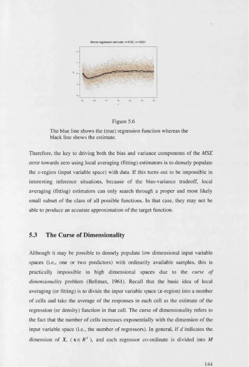
5.2 The Bias-Variance Tradeoff ... 140
5.3 The Curse of Dimensionality... 144
5.4 Defeating the Curse of Dimensionality... 146
5.5 The Loss of Interpretability... 146
6 Model Selection...150
6.1 Alternative Model Selectors... 150
6.2 Which Model Selector Should Be Used?...156
6.3 Extrapolation E rro r...160
7 Conclusion... 163
Appendices...167
Chapter 4
Homo Economicus as an Intuitive Statistician (2)
Bayesian Diagnostic Learning 1 Introduction...1722 Foundational Issues... 174
4 Bayesian Statistical Inference: A Wider View...190
5 Initial Bayesian Model Formulation... 193
5.1 Initial Data Model Specification...194
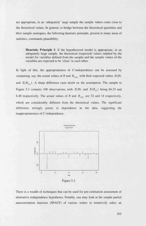
5.1.1 The Theoretical Approach to Data Model Specification 196 5.1.2 The Empirical Approach to Data Model Specification 199 5.1.2.1 The Independence Assumption...200
5.1.2.2 The Homogeneity Assumption...204
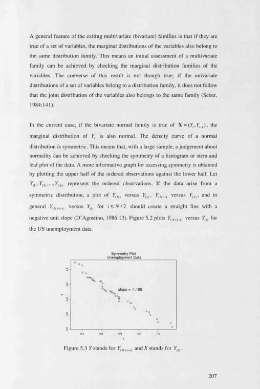
5.1.2.3 The Distribution Assumption...206
5.2 Prior Specification... 211
5.2.1 The Summary-Based M ethod... 211
5.2.2 The Hypothetical Prediction-Based Method...213
5.2.3 Default Priors...216
5.3 Some Limitations...219
6 Bayesian Empirical Model Assessment...221
6.1 A General Framework for Model Assessment...222
6.1.1 The Variety of Predictive Distributions... 224
6.1.2 Prior Predictive Checks... 225
6.1.3 Posterior Predictive Checks...229
6.1.4 Cross-validated Posterior Predictive Checks... 231
6.2 Bayesian Specification Searches... 234
6.2.1 Exploring Prior Distributions... 234
6.2.2 Exploring Data Model Assumptions... 240
7 Model Selection...243
8 Objections Revisited...247
9 Conclusion...251
Appendices... 256
Chapter 5
Homo Economicus as an Intuitive Statistician (3)
Data Driven Causal Inference 1 Introduction... 2602.1 Causal Structure... 263
2.2 Path Models... 266
2.3 Graphical Representation...268
2.4 Conditional Independence D ata...269
2.5 Assumptions Relating Probability to Causal Relations... 270
3 Causal Inference...274
3.1 Inference with Causal Sufficiency... 274
3.2 Inference without Causal Sufficiency... 277
4 Intrinsic Limitations of Data-driven Causal Inference... 281
4.1 Recursive Equivalent M odels...282
4.2 Non-recursive Equivalent M odels... 289
4.3 Causal Inference in Practice...292
5 Assumptions Revisited... 294
5.1 The Causal Markov Condition...294
5.1.1 Aggregation over Heterogeneous Units...296
5.1.2 Selection Bias... 300
5.1.3 Concomitants... 303
5.2 The Faithfulness Condition...306
5.2.1 The Measure Theoretic Argument... 306
5.2.2 Stable Unfaithfulness...310
6 Conclusion... 312
Appendices... 315
Chapter 6
The Economy as an Interactive System
An Appraisal of the Microfoundations Project 1 Introduction... 3312 The Representative Agent Modelling Approach...334
2.1 The Structure of the Representative Agent Approach...335
2.2 A Historical Example... 336
2.3 The Requirements of the Representative Agent Approach...339
2.3.2 Identical Aggregate and Individual Income Processes...345
2.3.3 Absence of Interaction among Economic Agents... 347
2.5 Problems with the Representative Agent Modelling Approach 350 3 Modelling Heterogeneous Behaviour...353
3.1 The Fundamental Theorem of Exact Aggregation...354
3.2 The Effect of Nonlinearity... 360
3.3 The Effect of Dynamics... 362
3.4 The Effect of Heterogeneous Environments...363
3.5 Heterogeneity and Policy Evaluation... 366
4 Modelling Interaction... 368
4.1 Market Interactions...369
4.2 Non-Market Interactions... 372
5 Conclusion...378
Appendices... 381
Finale
...392List of Tables
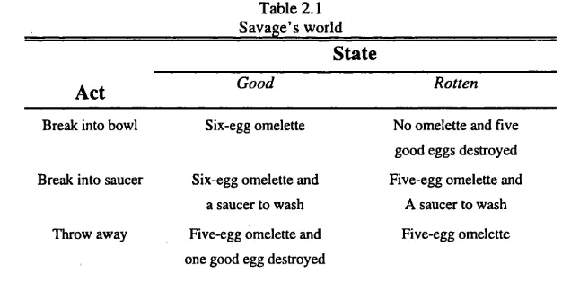
2.1 Savage’s Small World... 71
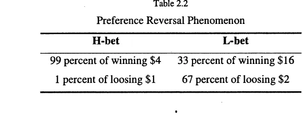
2.2 Preference Reversal Phenomenon...81
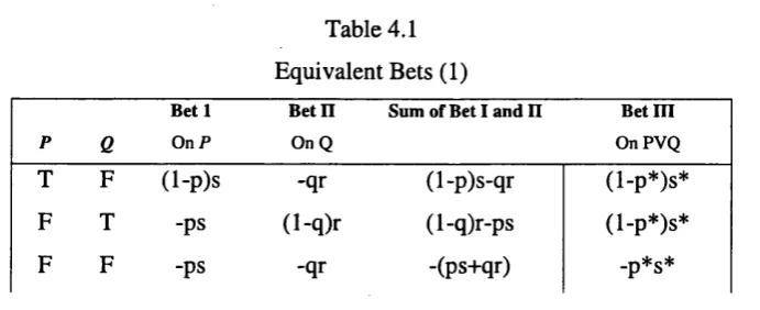
4.1 Equivalent Bets (1)... 176
4.2 Equivalent Bets (2)... 180
4.3 Definition of Vector of Interest...236
4.4 Normal AR(1) Model.1...237
4.5 Normal AR(1) Model I I ...239
4.6 Normal AR(2) Model... 241
4.7 Normal ARMA (1,1) M odel...242
Introduction
"As economics pushes on beyond 'static' it becomes less like science, and more like history." (Hicks, 1979: xi)
Modem economies consist of millions of heterogeneous decision-making units interacting with each other, facing different choice situations and acting according to a multitude of different mles and constraints. The interaction o f the decision-making units at the micro level gives rise to certain regularities at the economy level, which form the subject matter of macroeconomics. The complexity of modem economies makes it impossible to build an analytic model that represents the behaviour of all the basic decision-making units populating the economy. In modelling the economy, it is inevitably necessary to leave many details out, introduce aggregate variables, and focus on the relations among the aggregates. Macroeconomics is therefore primarily the study of aggregates.
The study of the economy at the aggregate level presents a number of difficulties. For practical reasons, the economy cannot be subjected to controlled experiments to establish causal relations true of economic aggregates. Economists have to rely on statistical analysis of aggregate data to study the causal relations true of the aggregates. Statistical analysis alone, however, is inadequate for causal inference, and must always be supported with substantive information regarding the underlying structure to yield new causal conclusions. Moreover, aggregate economic data are inherently imprecise, rendering the outcomes of statistical analysis in macroeconomics even more uncertain. These difficulties raise the issue of how it is possible in macroeconomics to acquire the non-sample information needed for modelling the structure of the economy.
thus makes a decision. Once we have established a theory o f behaviour, we can transform it into a theory of the economy as a whole using aggregation procedures. Since the theory is directly derived from the rules of individual behaviour, it correctly specifies the causal structure of the economy. Aggregate data can then be used to transform the theory into a quantitative model of the economy, describing the economic structure.
The enterprise of deriving the correct macroeconomic theory from microeconomic theory - or the microfoundations project - rests on two assumptions. The first is that we have, or it is possible to establish, an empirically adequate theory of individual behaviour. The other is that the theory can be transformed into a theory of the economy using aggregation procedures, without having to introduce any substantive assumption about the structure of the economy.
As regards individual behaviour, the basic idea in economics is that homo economicus follows the prescriptions of decision theory, understood in terms of one or another expected utility theory, in particular the theory of subjective expected utility. The theory of expected utility, in all the variants on offer, takes the agent’s view of the economy as given, and says nothing about how he predicts future values of economic variables. To fill this theoretical vacuum, new classical economists have set forth the rational expectations hypothesis, which identifies the agent’s subjective beliefs about the economy with the mathematical expectations implied by the true economic model. This gives rise to a view of the economy as a society in which everyone, except the econometricians, knows the structure of the economy. On this basis, the new classical paradigm defines economics as the enterprise to derive observable economic phenomena from two fundamental assumptions: (1) people are expected utility maximisers and (2) they maximise their expected utility with respect to the true model of the economy.
expectations economy by suggesting that, like econometricians, market participants also lack knowledge of the true economic model, and must learn it from available economic data. The new paradigm has been dubbed the bounded rationality paradigm, after Herbert Simon (1955, 1956). Though the idea of bounded rationality is relatively old, a unanimous interpretation of the paradigm is yet to emerge. One leading interpretation, set forth by new classical economists, conceives of the economy as a society of ‘intuitive statisticians’, where everyone, like econometricians, theorises, estimates, and adapts in attempting to learn about probability distributions that, under rational expectations, they already know (Sargent, 1993:3). So understood, the paradigm replaces the second principle of new classical economics with the assumption that agents maximize their expected utility with respect to models that, like econometricians, they construct from economic data. We will refer to the proposal that homo economicus behaves like an econometrician as the intuitive statistician hypothesis of bounded rationality.
This thesis studies several foundational issues relating to the theoretical approach to macroeconomics or, more specifically, the microfoundations project.
account. The contrast between these views reveals that the issues regarding theories of economic behaviour and those about the link between the micro and macro levels are the most basic topics in macroeconomics. Of equal importance is the conjecture that one can sensibly talk of structural relations at the economy level.
Chapter 2 studies the contribution of rational choice theories to economic theorising by concentrating on Savage’s theory of subjective expected utility. Using the framework of the theory, the chapter distinguishes between several phases of human decision making, which include (i) modelling the choice situation, (ii) defining the decision problem, and (iii) solving the problem. In light o f this, the chapter distinguishes between two possible types of theories of behaviour: choice-based theories of behaviour and learning-based theories of behaviour. The rational choice theories on offer fall into the category of choice-based theories of behaviour; they take for granted how the agent models his choice situation and defines his decision problem, and only explain how he solves a well-defined decision problem. So, in modelling behaviour using these theories, a host of substantive assumptions are needed to specify the agent view of his choice situation, and the problem he is trying to solve. These assumptions concern the agent’s view of the causal structure of the environment, his values, beliefs, needs, and goals.
The chapter then demonstrates that the resolution of economic controversies
ends with an analysis of the rational expectations hypothesis to explain why the hypothesis fails to eliminate the necessity of a learning-based theory of behaviour in theoretical economics.
Chapter 3 begins studying the intuitive statistician hypothesis. The usefulness of this hypothesis for modelling and thinking about the economy depends on whether there exists a ‘tight enough’ theory of statistical inference. To address this issue, the thesis proposes a preliminary conjecture about how a statistician perceives and models a choice situation: The statistician regards measurable features of the environment as realisations of some random variables, with an unknown joint probability distribution. He first uses the data on these quantities to discover the joint probability distribution of the variables and next uses the estimate of the distribution to uncover the causal structure among the variables. If the resulting model turns out to be inadequate, the initial set of variables is modified and the two phases of inference are repeated. This setting allows the separation of probabilistic inference issues from those of causal inference.
Chapter 4 studies the topic of statistical learning from the perspective of the Bayesian theory, which is said to allow the incorporation of background information into inference. The chapter first looks at some critical issues at the foundation of the Bayesian theory to explain why the theory, as stands, cannot be a theory of learning, and is only concerned with coherent analysis. As a result, to explain central aspects of inference such as model specification, empirical model assessment, and re- specification analysis, one has to go beyond the boundaries of the Bayesian theory. Having done this, the chapter draws on several themes in the relatively recent statistical literature to reconstruct a broader theory of Bayesian inference, which takes some steps in explaining the central aspects of inference traditionally left out in the Bayesian literature, including model formulation. Reflecting on the requirements and limits of the broader theory, the chapter considers the possibility of establishing a ‘tight enough’ theory of parametric inference, and brings to the fore some important implications for the bounded rationality program.
Chapter 5 studies the second phase of statistical learning relating to inference about causal structure. The chapter concentrates on the graph-theoretic approach to causal inference in order to investigate the possibility of a data-driven approach to causal inference. By data-driven we mean any effort to draw causal conclusions from probabilistic data using only general subject-matter-independent principles supposedly linking causation and probability. A claim for a data-driven approach to causal inference raises two separate issues. The first is whether there are universal principles connecting probabilistic and causal dependencies. The other is whether the principles are sufficient for inferring from the joint probability distribution of a set of variables the causal structure generating the distribution. The chapter takes up both topics, and by reflecting on the limits of data-driven causal inference outlines an account of causal inference from observational data.
Chapter 6 studies the other element of the microfoundations project that has to do with the move from a theory of individual behaviour to a theory of the economy. The chapter starts with a critique of the representative agent modelling approach to the study of the economy, explaining why understanding large-scale economic phenomena calls for thinking of the economy as a society of interactive heterogeneous individuals. Having done so, it investigates some basic issues that individual heterogeneity and interdependencies create for theoretical study of the economy. Individual heterogeneity and interdependencies existing in modem economies fundamentally undercut the conception of the economy underlying the microfoundations project. In fact, they sever any simple, direct, and useful link between the micro and macro levels, casting doubt on the very existence of stable relations at the economy level, which are suitable for a causal account.
The thesis concludes by highlighting some of the implications that arise from the chapters for the bounded rationality program in particular, and for the study of the economy in general. The marriage of the hypothesis that the agent behaves like a decision scientist with the hypothesis that he behaves like an intuitive statistician is not of much help in predicting the course of the economy.
Chapter I
Theoretical versus Atheoretical Macroeconomics
1
Introduction
Human beings in society have no properties but those which are derived from, and may be resolved into, the laws of the nature of the individual man. In social phenomena the Composition of Causes is the universal law (J.S. Mill, 1974 [1874]: 879).
The study of fluctuations in aggregate measures of economic activity and prices over relatively short periods (business cycle theory) and development of the economy over the long run (growth theory) constitutes what we call macroeconomics. The objective is to understand the causes of economic fluctuations and growth, forecast the future course of the economy, and aid analysis of state policies. Following tradition, we may categorise major objectives of macroeconomics under the headings of explanation, forecasting, and policy analysis. These objectives call for a quantitative model, which for most purposes must represent the causal structure of the economy. In macroeconomics, a major methodological issue is, therefore, the understanding of the causal structure of the economy.
A modern economy consists of millions of individual decision makers, firms, and institutions, each solving different decision problems under diverse circumstances and subject to distinct social and economic constraints. This complexity makes it practically impossible to build a model which represents the behaviour of all the basic decision making units of the economy. In modelling the economy, we inevitably need to leave out many details of the decision-making units, introduce aggregate variables, and focus on the relations of the aggregates. For this reason, macroeconomics is primarily the study of aggregates.
issue of how, in macroeconomics, we can acquire the subject-matter information necessary for a causal analysis of aggregate data.
There are two major reactions to these methodological limitations. On the one hand, there is the view that acknowledges the limitations involved in directly studying aggregate data but argues that they can be overcome indirectly. We can, so goes the argument, start by studying how individuals make their decisions, and thereby establish a theory of individual behaviour. Once we have established a theory of individual behaviour, we can transform it through aggregation into a qualitative theory of the economy. Having done this, with the help of statistical methods, we can use aggregate data to estimate the model parameters and thus establish a quantitative model. Since the model is derived from the rules of individual behaviour or other basic decision making units, it correctly specifies the causal structure of the economy, which is needed for the purposes of explanation and policy evaluation. We call this approach theoretical macroeconomics.
The other response argues that current theories of individual behaviour lack precision and substantial difficulties face any attempt to make them precise. Moreover, many complex issues arise in aggregating individual behaviour, relating to the heterogeneity of behaviour and interactions among decision makers. The aggregation difficulties rule out any simple relationship between the individual and the economy level, undermining the proposal of theoretical economics for establishing causal structure. Econometricians can build models that summarise economic data but cannot establish whether a model represents the economic structure. Aggregate data are also imprecise. This imprecision further weakens the reliability of macroeconomic models as'a tool for policy analysis. Economists must accept irresolvable differences among themselves and limit their claims to conclusions that follow from the analysis of imprecise aggregate data, which is the only objective ground in macroeconomics. We call this view atheoretical macroeconomics.
above two approaches to macroeconomics. The objective is to provide a glimpse of some basic controversies in macroeconomics and highlight the importance of the questions studied in this thesis.
This chapter is organised as follows: Section 2 defines macroeconomics, its subject matter and objectives. Section 3 discusses three arguments for the necessity of theory in macroeconomic analysis; all concern the boundaries of statistical analysis for causal inference. Section 4 sketches out the theoretical approach to macroeconomics, also known as the microfoundations program, and describes the assumptions underlying the program. Section 5 outlines the main features of the atheoretical approach and contrasts it with theoretical economics. Section 6 concludes with an outline of the issues studied in the thesis.
2
Macroeconomics
Macroeconomics studies recurring patterns discernible at the aggregate economic level, aiming to build a model that serves to explain why such patterns occur, predict their future developments, and analyse how policy interventions might affect them. This section first defines the fundamental notions of structure and structural model. It then characterises the objectives of macroeconomics and the features that a model should possess to serve as a means for achieving the objectives. In doing this, we follow the view of macroeconomics developed by the early econometricians working in the Cowles Commission.
2.1
Macroeconomic Structure
The variables used to describe an economy originate in the decisions made by its components - numerous individuals, firms, institutions, and governments.1 Families make decisions about what to consume and when, how many hours to work, and what
to invest in; firms make decisions about unemployment, production, pricing, marketing, borrowing, investment, and so forth. We can consider the input and output variables of these decision-makers as the basic variables of the economy. Often, the eventual outcome of the decisions is not quite what was planned: poor health may disrupt work, or a supply shortage may result in a lower production than expected. It is therefore sensible to model the decision outputs of an individual or institutional decision-maker as a function of its prominent input variables plus a stochastic residual vector. The vector of all input and output variables of all participants in the economy and their linking functions form the microstructure of the economy. We denote the microstructure by (m, r), where m and r stand for the vector of micro variables and micro-relations respectively. In place of (/n, r), the economic literature often refers to the triple (m, r, p) as the true economic data generating mechanism, where p is the joint probability distribution of the micro-variables m (Granger,
1990a:7; Hendry and Ericsson, 1991:18; Spanos, 1986:661-72).
The immense number of micro-variables and relations in any modem economy makes it impossible to consider the behaviours of all decision-making units in a model. Modelling an economy requires introducing aggregate variables and focusing on the patterns that emerge at the aggregate level. A central assumption in economics is that the microstructure (m, r, p) leads to a unique macrostructure (M, R, P), where M
stands for the set of aggregate input and output variables, R for the relations among the aggregates, and P for the joint probability distribution of the aggregate variables (Epstein, 1987:65). This macrostructure is the subject matter of macroeconomics. Thus, macroeconomics is defined as the study of the aggregative relations that emerge from decisions and interactions of the basic decision-making units of the economy. By contrast, microeconomics is defined as the study of the behaviour of the basic decision-making units of the economy in which no aggregation is involved. The presence of aggregation is what separates these fields of study from each other (Keynes, 1936:292-3).2
The above view of the subject matter of macroeconomics is consistent with mainstream economics that postulates the existence of recurring and stable relations at the aggregate level. However, there are several notions of macroeconomic structure and a host of views on the nature of the relation between the micro and macro structure. We continue by explicating a notion of structure found in the writings of the early econometricians working in the Cowles Commission, which will serve as a benchmark for defining alternative notions of structure and characterising some key controversies in macroeconomics.3
2.1.1 Structural Models
Early econometricians rarely defined the notion of structure explicitly. Instead, they focused on the related notion of structural model. It is convenient to first describe this notion and then use it to define the concept of structure. Consider the simple stochastic equation
Y = a + fiX + £, (2.1)
where Y is the response variable, X is the regressor, and £ is the error term with mean zero.4 This equation is commonly used to represent the regression of Y on X, giving the mean of the distribution of Y conditional on a particular value of X, i.e.,
E(Y I X = x) (Greene, 1990, ch.10). As a regression equation, (2.1) describes the association between X and Y in the population from which the data are sampled. As opposed to this usage, the equation may also be used for predicting the effects of (hypothetical) interventions in X on Y. If the equation correctly predicts how the values of Y change as we intervene to change the values of X, it is called structural
(Hurwicz, 1962:236-7). A difference between (2.1) as a regression equation and (2.1) as a structural equation is that in the former case the equation may cease to hold as
soon as changes are made to X whereas in the latter case the equation is invariant to interventions made to the values of X. Another way to state this notion of structural equation in the context of simple equation (2.1) is the following, which is borrowed with small changes from Pearl (2000:160):
Definition: An equation Y = a + pX + e is said to be structural if in an ideal experiment where we control X to x and any other set Z of variables (not containing X
or Y) to z, the value of Y would be independent of z and is given by a + fix + e.
This notion of structural equation captures the core of the manipulability conception of causation (Woodward, 1999). On this view of causality, variable X causes variable
Y if it is possible at least in a hypothetical experiment to change Y by manipulating X.
So, the claim that equation (2.1) is structural means that it expresses a causal relation. In that case, the parameter ft in (2.1) reflects the causal effect of X on Y, contrary to a regression equation in which ft only represents the degree of association between X
and Y in the population. The terms ‘structural’ and ‘causal’ are used interchangeably in what follows.5
Econometricians refer to the variables on the right hand side of a structural equation as exogenous', variable X in equation (2.1) is exogenous if intervening to set X = x
gives the same result for Y as observing X = x. Similarly, the variable on the left- hand side of a structural equation is called endogenous. Exogeneity also has weaker meanings in the literature. It sometimes refers to a variable whose value is not explained within the model but is supplied to it and sometimes refers to a variable which is statistically independent of the error term in the equation. We use ‘exogeneity’ to refer to the first notion, i.e., as an independent variable in a structural equation (Engle, Hendry, and Richard, 1983).
The early econometricians generalised the notion of a structural equation to systems of equations. An equation system forms a structural model if each equation in the
system is structural and remains invariant to changes that invalidate other equations in the model.6 In light of the definition of a structural equation as a causal relation, each equation in a structural model represents an autonomous causal mechanism that can be modified without undermining the mechanisms represented by other equations in the model. As an illustration, consider a simple version of the model of demand and price determination in economics, which has been discussed by many authors including Goldberger (1992) and Pearl (2000:27):
Q = ctx P + J3X 7 + £x (2.2a)
P = a 2Q + /12W + £ 2 (2.2b)
where Q is the quantity of household demand for product A, P is the unit price of A, I
is household income, W is the wage rate for producing A, and £x and £2 are error terms, representing unmodelled factors that affect quantity and price respectively. This model is structural if equation (2.2a) correctly forecasts the effects on Q of (hypothetical) interventions in P or 7, and equation (2.2b) correctly predicts the effects on P of interventions in Q or wage W. Moreover, interventions invalidating (2.2a) must not invalidate (2.2b) and vice versa.7 If we change the values of the parameters a x and /?, by intervening in the mechanisms determining the household income 7, the change must not affect a 2 and fi2. The mechanisms represented by these equations must be unrelated. In short, what makes this model structural is that each equation characterises an autonomous causal mechanism, one equation describing the causal process determining the demand for A and the other the process
o determining the price for A.
6 A broader notion of structural model is found in Koopmans (1949 [1971]).
7 A requirement necessary for this exercise is that £, be independent of P, £2 independent of Q, and
£{ independent o f £2.
This concept of structural model reveals the notion of structure implicit in the writings of the Cowles Commission econometricians. According to these researchers, a structure consists of a set of autonomous causal relations that can be utilised separately for intervening in the state of the economy. Koopmans, a leading member of the Commission, recapitulates this concept of structure in the following passage:
The study of an equation system derives its sense from the postulate that there exists one and only one representation in which each equation corresponds to a specific law of behaviour (attributed to a specific group of economic agents) ... Any discussion of the effects of changes in economic structure, whether brought about by trends or policies, is best put in terms of changes ip structural equations. For these are the elements that can, at least in theory, be changed one by one, independently. For this reason it is important that the system be recognisable as structural equations (quoted in Epstein, 1987:65).
From this perspective, the subject matter of macroeconomics is the study of autonomous causal relations true at the economy level, emerging from the interactions of individual decision makers with each other and with the environment. In what follows, we will refer to this viewpoint as the received view, and use it as a benchmark to define and compare some alternative views on the nature and scope of macroeconomics.
2. 2 Macroeconomic Objectives
To complete the description of the received view, it is also vital to expound on the objectives traditionally set for macroeconomics. This demands an understanding of the framework within which economic analysis is usually carried out. In its simplest form, consider an economy whose state at time t can be described by an endogenous variable Yt and an exogenous variable X t .9 The dynamics of the economy is described by a difference equation:
Yl+l= f ( Y (, X „ e , £ t ) (2.3)
where Q is a parameter vector defining the function /, and the disturbance term (random shock) £t has probability distribution P(£t). The description of the economy is completed by specifying the mechanism generating the exogenous variable X ,, shown by
X t =g( Z"A, e, ) (2.4)
where Z t denotes the only variable affecting X t, A a parameter vector defining the function g, and et a disturbance term with probability distribution Q(et) .10 The functions / and g are taken to be fixed but not directly known or at least not fully known. Data on X t and Yt is used to estimate 6 and A, as well as the parameters of the distributions P(£t) and Q(et). This fitted model is then used for prediction, policy analysis and explanation.
2.2.1 Prediction
Given an estimate of the parameters in the model (2.3), the task in prediction is to estimate the expected value of Yt+l when the values of Yt and X t are given. For the time being, the presence of Yt can be overlooked. Depending on how the value of X t
is given, three categories of prediction can be distinguished. First, there are cases where the actual value of X t is known and the model is used to predict Yl+l. Such predictions are called ex post predictions, since the actual value of X t is already
known. Secondly, there are cases where the actual value of X t is not yet known, and one instead uses guessed values of X t to predict future values of Yt . Such predictions
are called ex ante forecasts. In both ex ante and ex post prediction, one acts as an observer. Thus, if the model closely approximates the associations in the population during the periods for which the predictions are made, it will correctly forecast future values of Yt , regardless of whether it is structural or not.11 A regression model is sufficient for ex ante and ex post prediction, and no understanding of the causal mechanism generating Y and X is required.
Besides these types of predictions, the concern in economics is often conditional
prediction; that is, the objective is to predict the likely value y/+I that would arise if
X t could be set at a value different from its actual value. Since conditional prediction implies setting the values of an exogenous variable through intervention, the model must be structural or, in other words, invariant to the intervention to predict the outcome of the intervention. A regression model of the observed regularities is not adequate; one needs an understanding of the structure generating the data (Lucas and Sargent, 1979:298).
2.2.2 Policy Analysis
The objective in policy analysis is to design changes in the economy that take it to a desired state. In its simplest form, a policy consists of a change in the value of a policy variable, say X t , to alter the value of the target variable Y,+l ~ a policy variable is an exogenous variable whose values can be modified through state intervention. Analysis of such a policy involves predicting alternative values of Yt+i
that would arise if X t were set at values different from its actual value. If such predictions were possible, the future values of Yt could be estimated for various values of X t to find a value that would yield the desired result.
More often, a policy change is defined as a change in the mechanism that determines a policy variable. In the context of our simple economy, this concept of policy intervention amounts to a change in the mechanism
X t =g( Z„X, et). (2.4)
The underlying idea is that each set of possible values for the parameters X defines a possible mechanism for Xt . A policy change then consists of a change in the values of these parameters to influence the course of the economy (Tinbergen, vol.2 1939:18). The analyst considers a different set of values for X than the actual values to define an alternative mechanism for X t . Having done so, he uses the rule to generate a sequence of hypothetical values {xt } and recursively inserts them in the model (2.3) to simulate the course of the economy under the rule. The exercise is repeated for plausible values of X to select a rule with the desired outcome. A crucial requirement for the success of this exercise is that the model (2.3) remains invariant to changes in the policy rule (2.4). If a change in the mechanism generating X,
undermines the relation (2.3) that governs the behaviour of the endogenous variable
Yt , then an estimated version of (2.3) will not correctly predict the course of the economy under alternative policy rules (Lucas, 1976).
Policy analysis in either sense involves setting the values of the exogenous variables by intervention, and, for that reason, the relations in the model must be causal. Another equally important point is that if policy change involves a regime (rule) change, other relations in the model must be invariant to the modification in order to be of any use in predicting the policy outcomes. If one modifies equation (2.4), equation (2.3) must be invariant to the modification in order to be of any use in simulating the course of the economy.
2.2.3 Explanation
interest rate by 1% did not have the expected effect on the housing market. Still another concern, also related to policy analysis, is to understand the regularities that emerge at the economy level. To give an example, the Western economies post World War II displayed a trade-off between the rate of inflation and unemployment, known as the Phillips curve. The curve suggests that an increase in inflation is followed by a decline in unemployment. Any use of this regularity as a means for designing and evaluating employment policies demands understanding why the relation exists and, equally important, under what circumstances it may cease to hold. These queries fall under the general heading of explanation. We draw on some basic issues in the philosophical literature to find out what constitutes an adequate explanation of a particular fact. This will help us understand the features that a model should have in order to play a role in the explanation of economic phenomena.12
An early theory of scientific explanation, put forward by Hempel and Oppenheim ([1948] 1965), defines an explanation of a particular fact as an argument to the effect that the phenomenon to be explained was to be expected by virtue of certain explanatory facts (Hempel, 1965:336).13 The premises in the argument constitute the
explanans (that which does the explaining) and the conclusion is the explanandum
(that which is explained). Hempel requires that the explanans include at least one lawful generalisation. This view of explanation has become known as the inferential
view, since it identifies an explanation with an argument. Schematically an explanation in this approach takes the form:
True statements of initial conditions "I Explanans
Laws -*
Statement of what is to be explained. Explanandum
12 It is beyond the scope of this thesis to touch on the question o f what constitutes a satisfactory explanation of a law or regularity. A seminal paper on this topic is Friedman (1974). Chapter 6 can also be viewed as an exercise in explanation o f regularities.
Hempel distinguishes two models of explanation of particular facts. For contexts in which universal laws are available, such as the physical sciences, he proposes his deductive-nomological (D-N) model of explanation. A D-N explanation is a valid argument whose premises include at least one universal law and which deductively entails the explanandum. To give a well-known example, according to Hempel, we can explain why John has Down's syndrome by deducing the fact from the initial condition that John's cells have three copies of chromosome 21 and the law that any person whose cells have three copies of chromosome 21 has Down's syndrome. It is an essential characteristic of a D-N explanation that its explanans should include at least one lawful generalisation; accidental generalisation, Hempel says, do not explain.
For contexts such as macroeconomics in which generalisations are usually statistical, Hempel introduces his inductive statistical (I-S) model of explanation which proceeds by subsuming the event-to-be explained under a statistical law. An I-S explanation is also an argument, with the difference that its premises do not logically entail the explanandum, and are only required to confer a high probability on it. In a simple example from Hempel, if one asks why John rapidly recovered from his streptococcus infection, an I-S explanation is that he took a dose of penicillin, and almost all strep infections clear up quickly upon administration of penicillin. This, in Hempel’s view, forms an adequate explanation since the explanans are true and confer a high probability on the explanandum.
John's recovery is stated in terms of the class of people who take penicillin after having strep infection. In this class, the frequency of quick recovery from strep infection is high and thus, according to Hempel, we can explain John's recovery by the fact that he has taken penicillin. But this class can be partitioned into two subclasses: one subclass consisting of people with strep infection who are resistant to penicillin and the other consisting of those who are not. If John is a member of the former subclass, taking penicillin no longer explains his recovery, despite the fact that in both explanations the premises can be true. In general, an event is a member of many classes. Depending on the class chosen to subsume the event, we can explain the same event (John's recovery) with different degrees of probability, or even explain contradictory events (non-recovery). This raises the question as to how to choose a reference class to explain an event.
To address this question, Hempel adds that an I-S explanation must refer to a statistical generalisation that is stated in terms of a 'maximally specific' reference class to be satisfactory. By this, he essentially means that given our background knowledge it must not be possible to partition the class C in a nontrivial way that affects the conditional probability of the explanandum. To be precise, the class C is said to be maximally specific if the probability of the explanandum E is the same in any of its subclasses; that is, if P (E/ C,) = P (E/ C .) for any i and j, where
(C1,C2,...,CII) is any partition of C. According to Hempel, an I-S explanation is then adequate if the explanans are true, confer a high probability on the explanandum, and satisfy the requirement of maximal specificity.14
A problem with the maximal specificity requirement is that not all partitions affecting the probability of the explanandum are permissible. For example, given that John has lung cancer, that he has worked in a chemical factory where many employees have contracted lung cancer, that he has nicotine stained fingers, and that the frequency of lung cancer among people with nicotine stained fingers is higher, the requirement calls for using the statistical generalisation that provides the probability of lung cancer
among employees with nicotine stained fingers. But this partition is not permissible, since having nicotine stained fingers and having lunge cancer could be the effects of a common cause (heavy smoking), and an effect of a common cause does not explain another effect of the same cause. The moral of this story is that for an argument to be explanatory the explanans must be causally relevant to the explanandum. Mere statistical association is not sufficient (Salmon, 1998:309).
Another problem with the I-S model of statistical explanation is that it is symmetrical. Given a statistical association between Gaussian random variables X and Y which have no common causes, but X causes Y, the I-S model implies that one can explain X
by Y or Y by X. This implication goes against the intuition that, while causes explain effects, effects do not explain causes (Granger, 1988:17; Sobel, 1995:13). The conclusion is that the mere presence of a stable statistical correlation is not adequate for a statistical argument to be explanatory. An adequate explanation must relate the explanandum to its causes.
These considerations expose the difficulty of developing a theory of explanation of particular facts that makes no reference to causal relations. An explanation of a particular fact must give information relating to the causal process that has generated it. As Lewis (1986) notes, to explain a particular fact is to give information about its causal history. In general, whenever we try to explain a particular phenomenon, it must be shown that (1) the explanatory events are actually true, (2) the events are causes of the explanandum, in that if they were present and there were no preventative causes, the explanandum would occur too, and in addition (3) the events are actually the causes of the explanandum in the sense that if they had not been present in the situation under study the explanandum would not have occurred.15 The reason for the inclusion of this last condition is that for any event there might be > several sets of sufficient causes that could bring it about. Explanation of particular facts, therefore, calls for knowledge of the causal structure, and a model must be structural to be useful in explaining particular phenomena.
To summarise the received view of macroeconomics, there is a structure behind the aggregate data, consisting of autonomous causal relations that, at least hypothetically, can be manipulated independently of each other. The prime task of macroeconomics is then defined to be understanding and modelling of the structure. In addition, all the objectives traditionally set for macroeconomics, namely ex ante and ex post
prediction, conditional prediction, policy analysis and explanation, are considered as achievable.
3
The Need for Theory
A query for the received view is how the structure of the economy can be discovered. Natural sciences usually appeal to the method of controlled experiments to uncover causal relations. Economists are not in a position to subject the economic system to controlled experiments and must resort to statistical methods to analyse aggregate data. Yet, statistical analysis is inadequate for causal inference from sample data. There are three lines of arguments in the literature for this inadequacy of statistical methods, and hence the necessity of economic theory in macroeconomics. A brief study of these arguments sheds light on the reasons behind the emergence of competing approaches to macroeconomics.
3.1
Statistical Control
We first concentrate on the simple regression equation (2.1), and then extend the analysis to cases where there are several regressors involved. Since in the following the first moment of the variables is of no interest, we assume that the variables are measured around their mean, and drop the intercept from the equation. Equation (2.1) then becomes:
Y - fix + e (3.1)
Regression analysis is concerned with estimating the parameter f i, and the conditions under which an unbiased, efficient (minimum variance) and consistent estimate can be obtained from the data. To use this as a method of causal inference, one has to explain the conditions under which such an estimate of fi can be taken as an estimate of the effect of X on Y, as well as how the conditions can be established in practice. Accordingly, thee are three issues to address for a full view of the possible role of regression in causal inference. The first concerns the conditions under which an unbiased, efficient and consistent estimate of fi can be obtained from the data. The second concerns the conditions under which the estimate can be taken as an estimate of the effect of X on Y. Finally, the third concerns the possibility of establishing these conditions in practice. We will review the answers given to these questions by econometricians, and then explain why the regression method is unable to establish causation.
To estimate f i, users of the RMCI turn to the theory of ordinary least squares. This theory makes a number of assumptions about the error term e to ensure an efficient, unbiased and consistent estimation. To begin with, it assumes that the expected value of ei conditional on observation X ( is zero; that is, E{e / jc#) = 0 . This implies that
the unconditional mean E{e) is zero. Likewise, the same condition implies that ei
ensures that a least squares estimate of is unbiased. The theory also requires that observations on X provide no information about the variance and covariance of the error term £ . This means that the errors associated with the observations must have constant variance a 2 and be uncorrelated with each other. Under these conditions, a least-squares estimator of [5 is shown to be efficient, unbiased and consistent.
Econometricians and social scientists add one or two requirements to the orthogonality condition to identify an unbiased estimate of ft with the effect of X on
Y. Herbert Simon, in his celebrated article (1954), requires X to precede Y. By this, he intends to rule out bi-directional causation between X and Y. Others also require that
X can indeed be a causal variable so as to exclude nonsense inferences like inferring that having nicotine stains on one's finger causes lung cancer. Therefore, according to the users of the RMCI, a least squares estimate of the coefficient of X coincides with the effect of X on Y if X is uncorrelated with e, X precedes Y, and X can indeed be a causal variable. The validity of this answer, Simon maintains (1954), can easily be shown in the context of the simple regression equation (3.1). Suppose /? in (3.1) represents the effect of X on Y. If we multiply the equation through by X and take expectations of both sides, we will have
Cov(X, Y) = J3V(X) + Cov(X, e ), (3.2)
where Cov(X,Y) is the covariance of X and Y, V(X) is the variance of X, and
Cov(X,£) covariance of X and £. If X and £ are uncorrelated, the least squares estimate /3xy will be equal C o v ( X, Y) / V( X), which is the same as f i, the effect of
X on Y. That is,
However, if the condition fails, ftXY and /? will no longer be the same. Implicit in this analysis is that every correlation has a causal explanation, in the sense that it arises either because of a direct causal connection or because of unmeasured common causes. So, if the existence of unmeasured common causes is ruled out by assuming the orthogonality condition, a correlation between X and Y reveals the presence of a direct causal connection. Evidently, if the world contained spurious correlations, which could not be explained by reference to latent common causes, the orthogonality condition would not justify inferring from a correlation between X and Y that either X
causes Y or Y causes X. Such a conclusion would demand first ruling out all possible non-causal explanations.16
This brief description of the RMCI shows how the regression method is used to establish causation. Given the conditions, one simply regresses Y on X. If the least squares estimate fiXY differs from zero, X is said to cause Y, and if it is zero, X is said not to cause Y. The success of this method depends, on the one hand, on the adequacy of the conditions and, on the other, on the possibility of establishing them in practice. The first topic, that is, the adequacy of the conditions, falls outside the scope of this chapter.17 Instead, we study the second issue. All the three conditions demand a careful analysis. But, to keep the discussion short, we confine ourselves to an examination of the orthogonality condition, as this will suffice to explain why the RMCI fails.
The RMCI comes with a method for establishing the orthogonality condition. To explain the method, it is vital to note that this condition differs from other familiar statistical assumptions underlying a regression model, such as the linearity of the function linking X and Y or the normality of the distribution of Y. The validity of these assumptions can be checked by using observations on X and Y. In fact, for arbitrarily large samples, there are statistical algorithms that discover the functional
16 See N. Cartwright (1989) for a full discussion.
form of the relation between X and Y, and estimate the correct density function of Y.
In contrast, observations on X and Y contain no information on the validity of the orthogonality condition. This follows from the fact that the true disturbances £i
associated with observations (xity,) are never known. In practice, we can only estimate the residuals el =( y i —yi) % with yt being the predicted value of yr
However, if we use, for example, the least squares method to estimate /?, the residuals et are automatically uncorrelated with xr Thus, one cannot uses the residuals to establish the condition (Clogg, et al., 1997:94).18 In this sense, the condition is not a statistical assumption.
Faced with this limitation, econometricians have tried to establish, or at least support, the validity of the orthogonality condition by bringing in variables other than X and Y.
To understand the philosophy behind this attempt, one should note that the error term
£ in equation (3.1), when taken as a structural relation, stands for the effects of omitted variables on Y. Any correlation between X and £ is, therefore, said to indicate the presence of latent common causes for X and Y. Such variables are referred to as confounders.19 This interpretation suggests that the correlation between
X and £ can be eliminated by including all the confounders of X and Y in the regression of Y on X. In that case, the error term £ will be uncorrelated with X, and if other conditions are in place, an estimate of fi will coincide with the effect of X on
Y. It has thus been suggested that the orthogonality condition can be established by searching for all the confounders of X and Y, and including them in the regression of y on X. To estimate the effect of X on Y, it is not enough to estimate the simple regression equation (3.1). Instead, it is necessary to regress Y on X and all the confounders of X and Y. An estimate of the regression coefficient of X in this
18 The ordinary least squares regression coefficient of X is given by E(YX)/E(XX). If we define f t as equal to E(YX)/E(XX), we have
£ = Y — p X ,
X e = X Y - J3(XX),
E(X £ ) = E(YX) - p E { X X ) = 0.
equation corresponds with the effect of X on Y. The process of regressing on confounders is often called conditioning or statistical control.
The reasoning behind this claim can be illustrated by considering the case, where
0C\
there is only one confounder Z for X and Y. Suppose the process generating Y can be described by model (3.3):
X =qZ + £{ (3.3a)
y = p x + j z + e 2 ' (3.3b)
where Cov(ey, e2) = 0 , and a , f i, y are different from zero. Z in this model is a common cause of X and Y. If we estimate (3.1) in place of equation (3.3b), X and £
will be correlated, and a least squares estimate of the coefficient of X will differ from /?. To see this, we simply need to multiply (3.3b) through by X and take expectations of both sides to get
Co v ( X, Y) = j3V(X) + a j V ( Z ) .
We then have
* Cov(X,Y) pV( X) + a jV (Z)
V( X) V( X)
However, if Z is included in the regression of Y on X, the orthogonality condition is satisfied and the least squares estimate of ft can be equated with the effect of X on Y,
as shown below:
* _ Cov( X, Y/ Z) _ Cov( X, Y) V(Z)-Cov(X, Z)Cov(Y, Z) Pxy/z- V ( x f Z ) ~ V ( X ) V ( Z ) - C o v ( X , Z ) 2
P ( V ( X ) - a 2V(Z)) V ( X ) - a 2V(Z)
The example illustrates that regression on a confounder eliminates bias; it turns an otherwise biased estimate into an unbiased one.
The problem with this reasoning, of course, is that the set of confounders of X and Y
is not known. In practice, statisticians inevitably replace the set of confounders of X
and Y with a set of potential confounders, namely, a set of measured variables that precede X and Y and can possibly affect them. It is held that by controlling for potential confounders, one is likely to control for the real confounders, and eliminate possible correlation between X and e (Black, 1982:31). Thus, one is advised to control for as many potential confounders as one can to achieve a reliable estimate of the effect of X on Y. The longer the list of potential confounders included in the regression of Y on X, the more reliable is said to be the estimate:
One must include in the equation fitted to data every ‘optional’ concomitant [potential confounder] that might reasonably be suspected of either affecting or merely preceding Y given X - or if the available degrees of freedom do not permit this, then in at least one of several equations fitted to the data (Pratt and Schelifer, 1988:44).21
In this way, multivariate regression has come to dominate macroeconomics. To estimate the effect of X on Y, Y is regressed on X and a few other variables thought likely to affect both X and Y. The estimate of in the equation with all the potential confounders, whose inclusion affects the estimate of f3, is taken to represent the effect of X on Y. The RMCI can also be generalised to regression equations with multiple regressors. For a causal interpretation of a multivariate regression equation, all the regressors are required to precede the response variable Y and to be uncorrelated with the error term. Similarly, to establish the orthogonality condition,
one has to control for all the confounders of the regressors and the response variable (Clogg et al., 1997:94).
3.1.1 Limitations of Statistical Control
Critiques have questioned the adequacy of the RMCI from a variety of perspectives. Most of these criticisms relate to the limitations of statistical control in practice. One limitation arises from the small number of variables measured in practice. To state the critique precisely, let C be the complete set of potential confounders for X and Y. The plausible idea of statistical control is that if we could control for all the variables in C, we would be able to control for all the real confounders of X and Y, and estimate the effect of X on Y. But the set C is never completely known. What one measures in practice is a proper subset of C, which may exclude some or even all of the actual confounders of X and Y. As a result, conditioning on measured confounders can never guarantee the truth of the orthogonality condition, and a non-zero estimate of fi can always be due to latent common causes. The RMCI on its own fails to distinguish between cases of genuine causal connection and spurious correlation (Pearl, 2000:186).
Another problem is that conditioning on a measured variable, which is not a confounder but is taken as a potential confounder, can turn a consistent estimate of the effect of X on Y into an inconsistent estimate. This occurs whenever one controls for a barren proxy', that is, a variable Z that is correlated with factors that influence X
precedes both X and Y. Also, suppose that the causal structure of these variables is given by the model below (Figure 1),
X = U] + £x
Z — ccU, + U2 + £z
Y = j3X + )U2 + e y X Y Y = Death
U| = Smoking U2 = Age
Z = Nicotine stains X = Lung cancer
Figure 1
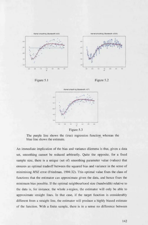
where £x, £z and £y are