Comparative Analysis of Brain Tumor Detection using Different Segmentation Techniques

Comparative Analysis of Brain Tumor Detection using

Different Segmentation Techniques

Ramaswamy Reddy, A., E.V. Prasad and L.S.S. Reddy

LBRCE, IT DEPT, JNTUK, Mylavaram A.P, India JNTUK, CSE DEPT, Kakinada, A.P, India

LBRCE, CSE DEPT, Mylavaram, India

ABSTRACT

In this study, we would like to present brain tumor detection methods, based on the conventional K-means technique, Expectation Maximization (EM) algorithm and a new Spatial Fuzzy-technique analysis of brain MR images. Though, the K-means and EM algorithm were already used in Brain MR image segmentation, as well as image segmentation in general, it fails to utilize the strong spatial correlation between neighboring pixels. A spatial Fuzzy C-means (SFCM’s) technique, which is utilize the spatial information properly and produce high quality segmentation of brain tumor images. Five ground truth images are taken to test the segmentation performance of K-means, EM algorithms and Spatial Fuzzy C-means technique. The segmentation results, which are proved more accurate segmentation by the SFCM’s compared to that of K-means and EM algorithm, are presented statistically and graphically.

Keywords

K-Means, Expectation Maximization, Fuzzy, MR images, SFCM’s

1.

INTRODUCTION

To locate specific object and boundaries in image, generally Image segmentation is used. A set of regions that collectively cover the entire image, or a set of contours extracted from the image will be the result of image segmentation. An important process of Segmentation is to extract specific and minute information from complex images. It has wide application in the field of medical science. With the application of image segmentation, we can split an image into mutually exclusive and exhausted regions such that each region of interest is spatially contiguous and the pixels within the region are homogeneous according to a predefined criterion. Generally, Brain images are complex and its nature is inhomogeneous, converting that inhomogeneous into homogeneous is very difficult. Without image segmentation, it is very difficult to visualize the structure of the image for neurologists or radiologists. Hence, there is requirement of automatic segmentation techniques for brain MR images. This study deals with the concept of automatic brain tumor segmentation. Normally the anatomy of the Brain can be viewed by the MRI scan or CT scan. In this study the MRI scanned image is taken for the entire process. The MRI scan is more comfortable than CT scan for diagnosis. It will not affect the human body and there will be no radiation, because it is based on the magnetic field and radio waves.

Actually, tumor forms due to the uncontrolled growth of the tissues in any part of the body. We find two kinds of tumors like Primary or secondary. Secondary tumor means spreading of existing tumor to another part of the body and grown as its own. Generally, Cerebral Spinal Fluid (CSF) is affected by the brain tumor and it causes Strokes. The treatment is given for the strokes rather than the tumor. For that treatment, the detection of tumor is essential. Naturally, tumors are malignant and mass. Mass tumor detection is easy, where as it is a little bit difficult

to locate the malignant tumor .There are different types of algorithms used for brain tumor detection.

In this study, we have analyzed different types of algorithms for the detection of brain tumor. These algorithms are developed by using Mat Lab. It is easy for the development and execution. Finally, we have found out the methods for tumor detection and exact location of the tumor with accurate boundaries.

1.1.

Literature Survey

The Magnetic Resonance Imaging (MRI) is a highly acceptable means than Computed Tomography (CT) to acquire high-resolution images of the brain of live subjects. Due to accuracy and soft tissues of brain contrast allows the discrimination of the nerve connection from the congregations of neurons and Cerebrospinal Fluid (CSF) (Ahmed and Iftekharuddin, 2011). To support the diagnosis of various brain illnesses such as Alzheimer’s disease, Dementia with Lowy bodies and Parkinson’s disease, we need the analysis of the spatial distribution of those tissues.

Previously, some of the methods like-manual slice editing, region painting and interactive threshold are used for medical image segmentation, which depends on human graphical interaction to define regions of interest. The different methods of image segmentation are classified into four main categories by Yong yang et al.(2007) (1) Threshold region growing and edge based techniques which are considered as classical methods. (2) The Maximum-Likelihood Classifier (MLC), which comes under statistical method. Basically, these methods are supervised and depend on the prior model and its parameters. André michael coleman(june 2008) found out reasonable opening results with Bayesian MLC. proved the superiority of the neural network by making comparison between the MLC and the neural network classifier. From the last few years, some new methods of segmentation have been introduced, that could be classified as Statistical methods.

Transverse, Coronal and Sagittal MRI slices map in three directions which include in the brain MRI. Amongst, T1-weighted image, T2-T1-weighted image and PD-T1-weighted image are the three modes of the transverse slice mapping. Generally, high contrast and low noise characteristics consisting of T1 weighted MRI image, so that T1-weihted image segmentation algorithms are widely used. The accuracy of the multi-spectral image segmentation can often be higher than that of the single-channel image segmentation, because, multi-spectral images composed by different modes are usually able to provide richer anatomy information. Multi-spectral image processing algorithms are usually more complex than the single-channel image processing algorithms, because the different modes have their own unique characteristics and different processing methods.

2.

MATERIALS AND METHODS

2.1.

K-Means Algorithm

K-means is a heuristic method and conventional, which gives better output in data clustering. “K-means clustering is an interactive procedure”. The K-means clustering technique group the information by repeatedly finding the statistical mean value for each group after segmenting the image through classifying each pixel in the group with nearest mean. The steps concerned in the K-means algorithm are given below:

1. Select K initial clusters z1(l),z2(l),………..zK(l)

2. The Kth recursive step, take the samples between k clusters given below xCj(k) if ||x-zj(k)||<||x-zi(k)|| For i

= 1,2,………..,k, i≠j, where, Cj(k) denotes the deposit of

samples whose cluster center is zj(k)

3. Obtain the new cluster centers zj(K+1), j =

1,2,………….,k, such that the Euclidean distance from points in Cj(K).Therefore, the innovative cluster is given

by:





j

i _{x C}

j 1

Z k 1 x

N 

 



number of samples in Cj(k)

If zj(k+1), j = 1,2,..,k, the computation will be converged

at the end else go to step 2

After segmentation of brain MR image, we can find out boundaries of the image using canny edge detection. After that, we find out labeling of the image and finally exact location of the tumor in the image.

Advantages of K-means technique are:

 There are always K clusters

 There is always at least one item in each cluster

2.2.1.

Data Modeling

Generally, the image data is used to represent by statistical models, which consider the image as a random process in particular or a mixture of random processes. The most suitable example for the random processes is a Gaussian distribution function, which is assumed to be represented by independent identically distributed functions (iid’s). The representation of the model is (Boccignone G,et. al, 2005):









i _{k 1} k i k

f x | 



Here, the representation of K is the number of processes or classes that need to be extracted from the image, k ∀ k = 1, 2, 3,…, K. The form of the parameter vector of class k is [µk, σk] such that µk is the mean and σk is the standard deviation of the distribution K, pk is the mixing proportion of class k (0<pk<1,

∀ k=1,….., K and kpk = 1, the intensity of pixel i is xi and Ф={p1,…., pk, µ1,…., µk, σ1,..., σk} is called the parameters vector of the mixture (Ambroise and Govaert, 1996).

The missing data that defines the mixture is represented by the parameter vector Ф. The maximum log-likelihood estimator is utilized by the EM algorithm to estimate the value of Ф (Hsu, 1997) Consider:

 









1 2 n t 1 i

L  f x , x ,...x | 



If Ф is the true value of the parameter, the joint probability distribution, L(Ф) represents the likelihood that the values x1,x2,…., xn will be observed. The maximum value of L(Ф) which is defined in ФML, as:

 



 



L arg max L  (3)

Here, ФML denotes the maximum log-likelihood estimator of Ф.

2.3.

The Algorithm of Expectation and

Maximization

Each pixel of the class in the image can be easily determined after the values of the parameters are found by computing the probability of this pixel to be belonging to each class in the image. The unknown parameters of a mixture model are found by using the EM algorithm that maximizes the log-likelihood of the sample.

2.4.

The Steps of the EM Algorithm

EM algorithm which is attained by performing two steps iteratively.

2.5.

The Expectation (E) Step

2.6.

The Maximization (M) step

In this step, actually measured data by using the data from the expectation step as shown below:





N _t

ik i

( t 1) i 1

K N t

ik i 1

2

N t t 1 N t

ik i ik

2 t 1 i 1 t 1 i 1

K N _t ik i 1 Z x Z

Z x Z

k p N Z                











The criterion is alternatively optimized by the each iteration of the EM algorithm, with the parameters Ф fixed, according to the parameters of the mixture with a fixed pixel class probabilities and then according to the pixel class probabilities Z = [Zik]. The starting of the EM is initial estimation of the parameters of the distributions and the proportions of the distributions in the image Ф (0).

The EM algorithm producing the missing parameters, that is Ф, which is always followed by a classification step and then those parameters are used by a classifier which we define it as:









i i k

k arf max G x , (6)

It assigns a class membership to a pixel i depending on its intensity, xi, to the class which its parameter vector maximize the Gaussian density function.

2.7.

The EM Algorithm steps

The steps of EM algorithm for image segmentation are as follows:

 The system consisting of the number of classes K and the image I.

 Based on the histogram of the image and the number of classes, Ф(0) is initially estimated. For example, a general guess for the means and variances for the three classes (WM, GM and CSF) are required for MRI segmentation. Highest mean consisting of White Matter and lowest mean consisting of CSF. The histogram of the image should be used, due to the variation between different MRI acquisition systems. The priori class probabilities pk are

understood to be equally likely.

 Iteratively performing the E-step and M-step until convergence, the E-step compute the class probability of each pixel at each iteration based on the current estimation of Ф(t)_{. The new expectation of Ф}(t+1)

is determined in M- step, based on values of E-step. The maximum estimator of Ф is produced after convergence

 To generate the classification matrix C, use ФML in a classifier

 Based on the classification matrix C assigns color or label to each class then the segmented image is generated.

After segmentation of brain MR image, we can find out boundaries of the image using canny edge detection. After that, we find out labeling of the image and finally exact location of the tumor in the image.

Advantages of EM algorithm:

 It reduces the computational complexity of the segmentation

 It allows the use of the well characterized Gaussian Density function

The limitations of EM algorithm:

 It fails to utilize the strong spatial correlation between neighboring pixels

 All the pixels are identical and independently distributed (Boccignone G,et. al, 2005)

2.8.

Fuzzy C-Means Clustering (FCM)

Fuzzy-C means is automatic technique that has been effectively used in MR images for the target identification and segmentation of images. The Fuzzy C-means technique labels the pixels by individual sets of data values into clusters. The fuzzy segmentation methods keep additional data from the innovative images than solid segmentation techniques (Pham, 2003). Fuzzy C-means is obtained based on Fuzzy pixel classification into particular regions, which are belongs to one class of pixels. FCM allows pixels to fit into various classes having unreliable degrees of membership. This type of analysis gives simple performance in a number of real time segmentation which is used regularly in MRI (Christ,C.J.et.al,2011). The degree of membership is used to collect pixels with good value of classification.. This helps the surface to convergence at the peaks of membership function. The inhomogenity object is not carried in the entire medical (Kannan, 2005; Alizadeh et al., 2008).

The Fuzzy C-means (FCM) is a process of partition the one portion of information from two or more parts. The minimization of object function is given by:

N c m 2

ij j i

j 1

J

 

Here, uij indicates Membership function of pixel xj within the ith cluster, vi indicates ith cluster center and m is the uncertainty value which is taken as 2.

The cost function is decreased when pixel is near to centroid, which have high values of membership function and minimum values of membership function are allocate to far pixel from the centroid. Thus, the membership function gives probability of pixel belongs to particular cluster. The algorithm dependants on the measure of distance between pixel and individual cluster having the centriod in the feature domain of the image.

The degree of membership function and cluster centers are generated every time with new values by using equation:

ij 2

m 1

c j i

k 1

j k

1 || x v || || x v ||

          _   



i N m

j 1 ij

u xj V u   





the same cluster is enormous though, this spatial relationship is significant in clustering, it is not applied in a classical FCM algorithm.

2.9.

Spatial FCM

The arrangement of pixels in spatial domain is given to develop spatial domain information as:

j

ij K NB ik

h 



where, NB(xj) denotes the square kernel centered on pixel xj in the image. A 33 kernel is implemented in this procedure. Here, the function hij represents the chance of getting the pixel xj belongs to ith cluster. The hij of a pixel for a cluster is large when the majority of its neighborhood having the similar cluster. The hij is introduced into membership degree as follows:

' p q c p q

ij ij ij k 1 kj kj

u u h /



p and q are relative parameters. These parameters organize the relative importance of both variety functions. In the area of homogeneity, the hij fortify the real membership and the clustering results remain constant. However, in the case of a pixel with noise, this equation reduces the value of a noisy cluster by the labels of its mask pixels. Thus, mismatching classified pixels from noisy regions or false blobs can be rejected. The clustering is a two sided process. In the first iteration, the membership function in the frequency domain is calculated. In the second iteration, degree of the membership function of each pixel is mapped to the pixel domain and the hij is then evaluated. The FCM iteration continues with a fresh membership function until the solution converges. The iteration halts when the difference between two cluster going maximum for two successive repeation process is less than a threshold (Є = 0,02). Finally, the solution is converged, defuzzification is

implemented to assign pixel to a particular cluster for which the degree function is maximal.

After segmentation of brain MR image, we can find out boundaries of the image using canny edge detection. After that, we find out labeling of the image and finally exact location of the tumor in the image.

Advantages of FCM technique:

 It provides more detailed information than classical “hard” classification

 The classes number can be defined in conventional process can be less than unsupervised classification

 Limitations of FCM technique:

 The selection of parameters p and q for each brain MR image is difficult

 The handling of outliers is difficult

3.

EXPERIMENTAL RESULTS

In MATLAB simulation, two brain MR images are considered for validating the proposed algorithm. These images are generated using Fuzzy C-means algorithm. The performance of the algorithm is compared with K-means and Expectation and Maximization methods in terms of noise, quality metrics and time complexity of each brain MR images.

Signal to Noise Ratio (SNR) is defined as:

i

dB 10 2 i 2

1 x

SNR 10log

N

 

 _{ }



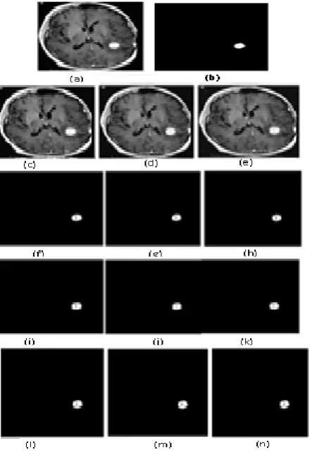
Figure. 1 Image segmentation of brain MR image of size (165175)-(a) original image and (b) ground truth tumor image, (c), (d) and (e) Gaussian noise images with 3, 5 and 7% respectively; (f), (g) and (h) corresponding segmented tumor

images using k-means method respectively; (i), (j) and (k) corresponding segmented tumor images using Expectation Maximization respectively; (l), (m) and (n) corresponding segmented tumor images using Spatial

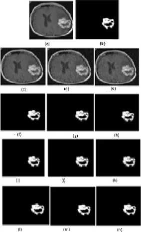
Figure. 2 Image segmentation of brain MR image of size (165175)-(a) original image and (b) ground truth tumor image , (c), (d) and (e)Gaussian noise images with 3, 5 and 7% respectively; (f), (g) and (h) corresponding segmented tumor

images using k-means method respectively; (i), (j) and (k) corresponding segmented tumor images using Expectation Maximization respectively; (l), (m) and (n) corresponding segmented tumor images using Spatial

Table 1. The error rates of first brain MR image of size (165  175) with SNR 3, 5 and 7% obtained by K-means algorithm, Expectation Maximization algorithm and Fuzzy C-means corresponding to Fig. 1(a)

Error rates

--- Expectation Fuzzy Noise levels % K- means maximization c-means

3 3.78 2.89 2.01

5 4.67 3.91 3.23

7 6.21 5.71 4.88

Fig 3: The first brain MR image segmentation with tumor error rates obtained by K-means, Expectation and Maximization methods with different levels of noise using Table 1.

Table 2. The error rates of second brain MR image of size (165  175) with SNR 3, 5 and 7% obtained by K-means algorithm, Expectation maximization algorithm and Fuzzy c-means corresponding to Fig. 2(a).

Error rates

--- Expectation Spatial Noise levels% K-means maximization Fuzzy

3 3.65 2.06 1.75

5 4.06 3.06 3.09

7 6.13 5.23 4.36

Fig. 4. The second brain MR image segmentation with tumor error rates obtained by K-means, Expectation and Maximization method and Spatial Fuzzy technique with different levels of noise using Table 2

The segmentation performance is evaluated by using objective segmentation evaluation criteria based on Jaccard Index (JC), Volumetric similarity (VC), Global Consistency Error (GCE), Variation Of Index (VOI) and Probability Random Index (PRI) formulas are given below:

Consider X and Y as given ground truth tumor and output tumor images:

| X Y | a

JC

| X Y | a b c



 

   (13)

|| X | | Y || b c

VC 1 1

| X | | Y | za b c

 

   

  

Where:

X Y

a | X Y |, b ,c ,d X Y

Y X      

 













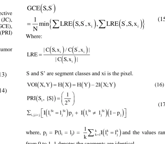
GCE S,S

1

min

LRE S,S , x ,

LRE S ,S, x

N







Where:

  



 

| C S, x |



S and S’ are segment classes and xi is the pixel.





 

 





VOI X,Y H X H Y – 2I X;Y (16)















t N

St St St St

i, j,i j i j j i j j

1 PRI S , {S}

2

I l l p I l l 1 p

     _{ }    _     _ (17)

where, pj = P(li = lj) =





k k k

k 1 i j

1

I l l

k



0 2 4 6 8

3% 5% 7%

Y -axi s Er ro r R ate s

X-axis: Different Noise Levels

K-Means Expectati on Maximiza tion 0 1 2 3 4 5 6 7

3% 5% 7%

Y --axi s-:E rr o r R ate s

X-axis : Different Noise Levels

K-Means

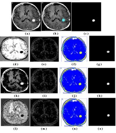
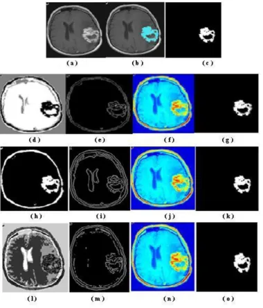
Fig. 5: Image segmentation of the first brain MR image of size (165175) - (a) Original image; (b) and (c) are ground truth and ground truth tumor images respectively; (d), (e), (f) and (g) are images with segmentation, boundary, label and

tumor segmentation respectively of K- means method; (h), (i), (j) and (k) are images with segmentation, boundary, label and tumor segmentation respectively of Expectation Maximization method; (l), (m), (n) and (o) are images with

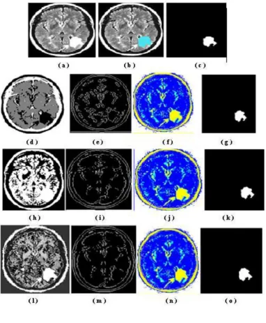
Fig. 6: Image segmentation of the second brain MR image of size (165175) - (a) Original image; (b) and (c) are ground truth and ground truth tumor images respectively; (d), (e), (f) and (g) are images with segmentation, boundary, label

and tumor segmentation respectively of K- means method; (h), (i), (j) and (k) are images with segmentation, boundary, label and tumor segmentation respectively of Expectation Maximization method; (l), (m), (n) and (o) are

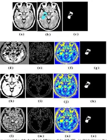
Fig. 7: Image segmentation of the third brain MR image of size (165175) - (a) Original image; (b) and (c) are ground truth and ground truth tumor images respectively; (d), (e), (f) and (g) are images with segmentation, boundary, label and

tumor segmentation respectively of K- means method; (h), (i), (j) and (k) are images with segmentation, boundary, label and tumor segmentation respectively of Expectation Maximization method; (l), (m), (n) and (o) are images with

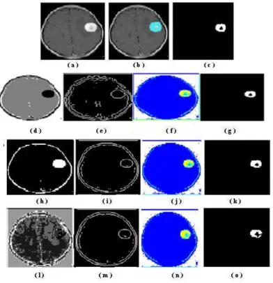
Fig. 8: Image segmentation of the fourth brain MR image of size (165175) - (a) Original image; (b) and (c) are ground truth and ground truth tumor images respectively; (d), (e), (f) and (g) are images with segmentation, boundary, label

and tumor segmentation respectively of K- means method; (h), (i), (j) and (k) are images with segmentation, boundary, label and tumor segmentation respectively of Expectation Maximization method; (l), (m), (n) and (o) are

Fig. 9: Image segmentation of the fifth brain MR image of size (165175) - (a) Original image; (b) and (c) are ground truth and ground truth tumor images respectively; (d), (e), (f) and (g) are images with segmentation, boundary, label and

tumor segmentation respectively of K- means method; (h), (i), (j) and (k) are images with segmentation, boundary, label and tumor segmentation respectively of Expectation Maximization method; (l), (m), (n) and (o) are images with

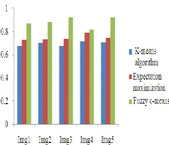
Fig. 10. Jaccard coefficient for five different brain MR image segmentations using K-means, Expectation and maximization and Fuzzy c-means algorithm using Table

Fig. 11. Volumetric similarity for five different brain MR image segmentations using K-means, Expectation and

maximization and Fuzzy c-means algorithm

Fig. 13. Global Consistency Error for five different brain MR image segmentations using K-means, Expectation and

maximization and Fuzzy c-means algorithm

Fig. 14. Probability Random index for five different brain MR image segmentations using K-means, Expectation and

maximization and Fuzzy c-means algorithm

Fig. 12. Variation of Index for five different brain MR image segmentations using K-means, Expectation and

3.1. Discussions

Two different Brain MR Images as shown in Fig. 1 and 2 are considered to validate the algorithm. The first brain MR image of size (165175) is shown in Fig. 1. The Gaussian noise images of SNR 3, 5 and 7% are shown respectively in the Fig. ( c ) , (d) and (e) and the correspnding numerical values are given in Table 1. By applying K-means algorithm on these brain MR images, the results thus obtained are shown respectively in Figures (f), (g) and (h) and the corresponding numerical values are given in Table 1.

It is observed that the performance of the algorithm gradually deteriorates with increase in noise strength. Similar observations are also made in the case of Expectation and Maximization (EM) Method. The results obtained by EM Method are shown respectively in Figures (i), (j) and (k) and the corresponding numerical values are given in Table 1. Here also, the performance of the algorithm gradually deteriorates with the increase in noise strength. The results obtained by applying Fuzzy C-means method on these brain MR images are plotted respectively in Figures (l), (m) and (n) and the corresponding numerical values are given in Table 1. In this method also, the

performance of the algorithm gradually deteriorates with the increase in noise strength, however, the segmentation results are more accurate and acceptable as compared to those obtained by the K-Means and Expectation Maximization.

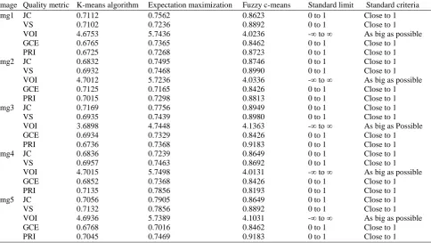
The Table 3 and corresponding Fig. 10 through 14 shows that K-means method gives 70 to 72% of accuracy in all the cases of five brain MR images while the Expectation and Maximization method gives 72 to 79% of accuracy and Fuzzy C-means gives 81 to 91% of accuracy in all the cases of five brain MR images respectively. From the above segmentation quality metrics, it can be clearly seen that the model developed by using Fuzzy C-means algorithm gives better results than K-means and Expectation Maximization methods and percentage improvement in segmentation quality is from 4 to 10.

The time complexity of each of these methods is also determined. It is observed that the time complexity decreases in the case of Fuzzy C-means algorithm as compared to that of K-means method and Expectation and Maximization method. The corresponding values are respectively 0.6207, 0.81620 and 0.92000 sec.

Table 3. Segmentation results of quality metrics using K-means, expectation maximization method and fuzzy c-means algorithm for five different brain MR images

Image Quality metric K-means algorithm Expectation maximization Fuzzy c-means Standard limit Standard criteria

Img1 JC 0.7112 0.7562 0.8623 0 to 1 Close to 1

VS 0.7102 0.7236 0.8892 0 to 1 Close to 1

VOI 4.6753 5.7436 4.0236 -∞ to ∞ As big as possible

GCE 0.6765 0.7365 0.8462 0 to 1 Close to 1

PRI 0.6725 0.7268 0.8723 0 to 1 Close to 1

Img2 JC 0.6832 0.7495 0.8746 0 to 1 Close to 1

VS 0.6932 0.7468 0.8990 0 to 1 Close to 1

VOI 4.7012 5.7236 4.0336 -∞ to ∞ As big as possible

GCE 0.7125 0.7165 0.8426 0 to 1 Close to 1

PRI 0.7015 0.7298 0.8813 0 to 1 Close to 1

Img3 JC 0.7169 0.7756 0.8949 0 to 1 Close to 1

VS 0.6935 0.7439 0.8980 0 to 1 Close to 1

VOI 3.6898 4.7448 4.1363 -∞ to ∞ As big as Possible

GCE 0.6934 0.7329 0.8426 0 to 1 Close to 1

PRI 0.6736 0.7368 0.9183 0 to 1 Close to 1

Img4 JC 0.6836 0.7239 0.8649 0 to 1 Close to 1

VS 0.6957 0.7463 0.8692 0 to 1 Close to 1

VOI 4.7015 5.7498 4.0131 -∞ to ∞ As big as possible

GCE 0.6852 0.7368 0.8426 0 to 1 Close to 1

PRI 0.7135 0.7856 0.8193 0 to 1 Close to 1

Img5 JC 0.7056 0.7905 0.8649 0 to 1 Close to 1

VS 0.7132 0.7856 0.8892 0 to 1 Close to 1

VOI 4.6936 5.7389 4.1031 -∞ to ∞ As big as possible

GCE 0.6768 0.7016 0.8462 0 to 1 Close to 1

[3] André michael coleman, June 2008. Dissertation: An adaptive landscape classification procedure using Geoinformatics and artificial neural networks, faculty of earth and life sciences Vrije universiteit, Amsterdam The Netherlands.

[4] Vannier, M.W., C.M. Speidel and D.L. Rickman, 1991. Validation of Magnetic Resonance Imaging (MRI) multispectral tissue classification. Comput. Med. Imaging Graph, 15: 217-223. PMID: 1913572

[5] Matthew Deighton and Maria Petrou, 2003. supervised segmentation of Volume Textures using 3D Probabilistic Relaxation. SCIA,LNCS 2749,pp 869-876. Springer-Verlag Berlin Heidelberg.

[6] Shweta Jain, Shubha Mishra, 2013. ANN Approach Based On Back Propagation Network and Probabilistic Neural Network to Classify Brain Cancer. (IJITEE) ISSN: 2278-3075, Volume-3, Issue-3,pp: 101-105.

[7] Shan Shen, William Sandham, Member, IEEE, Malcolm Granat, and Annette Ster. MRI Fuzzy Segmentation of Brain Tissue Using Neighborhood Attraction With Neural-Network Optimization. ieee transactions on information technology in biomedicine, vol. 9, no. 3, september 2005

[8] Chuang, K.S., H.L. Tzeng, S. Chen, J. Wu and T.J. Chen, 2006. Fuzzy c-means clustering with spatial information for image segmentation. Comput. Med. Imaging Graph., 30: 9-15. PMID: 16361080

[9] Indah, S., S. Adhi, S.W. Thomas and T. Maesadji, 2011. MRI brain images segmentation based on optimized fuzzy logic and spatial information. Int. J. Video and Image Proc. Netw. Secu., 11: 6-6.

[10]Boccignone G, Napoletano P, Caggiano V, Ferraro M. 2005 A multiresolution diffused expectation-maximization algorithm for medical image segmentation. Comput Biol Med. 2007 Jan;37(1):83-96.

[11] Saeed, M., W.C. Karl, H.R. Rabiee and T.Q. Nguyen, 1998. A new multiresolution algorithm for image segmentation. Proceedings of the IEEE International Conference on Acoustics, Speech and Signal Processing, May 12-15, IEEE Xplore Press, Seattle, WA,pp:2753-2756.

[12] Pham, D.L., 2003. Unsupervised tissue classification in medical images using edge-adaptive clustering. Proceedings of the 25th Annual International Conference of the IEEE Engineering in Medicine and Biology Society, Sep. 17-21, IEEE Xplore Press, pp: 634-637.

[13]Christ,M.C.J. Parvathi, R.M.S. 2011 Fuzzy c-means algorithm for medical image segmentation Electronics

Computer Technology (ICECT), 3rd International

Conference on (Volume:4,pp:33-36).

[14] Kannan, S.R., 2005. Segmentation of MRI using new unsupervised fuzzy C mean algorithm. ICGST-GVIP J.