Design and Implementation of Speed Controller with Anti Windup Scheme for Three Phase Induction Motor Used in Electric Vehicle

Design and Implementation of Speed Controller with

Anti-Windup Scheme for Three Phase Induction Motor

Used in Electric Vehicle

Prasun Mishra

QHS (T)

CSIR-CMERI, India

ABSTRACT

Design of reliable and robust controller for electric vehicle in urban and sub urban areas is very much challenging task due to time varying load torque requirement at the wheel of the vehicle. In this paper indirect field oriented vector control of induction motor, PI speed control with anti-windup scheme and hysteresis current control scheme have been proposed for three phase induction motor drive train and simulated in MATLAB Platform. For its hardware implementation, a laboratory level experimental set up has been build up and the control logic has been tested successfully by performing a no of experiments at different operating conditions.

Keywords

Electric Vehicle, Three Phase Induction Motor, IFOC, Anti-windup PI controller, Hysteresis Current Controller

1.

INTRODUCTION

The use of IC engine in the ever increasing fleet of world vehicles has been questioned in recent times due to the increasing concerns of global warming. Battery operated Electric vehicle [1], [2] is the best solution to mitigate this environmental pollution, particularly in large urban and sub-urban areas. In medium weight electric vehicles designed for typical urban and sub urban areas, frequent accelerations and decelerations can occur because of the huge traffic, signal lights and other road conditions. These accelerations and decelerations form the intermittent parts of the load, while the friction and air drag form the continuous parts of the load for the drive motor [3], [4]. So a robust speed controller has to be designed for the propulsion motor to cater to the requirements of time varying characteristics of road load to run the vehicle efficiently, reliably and safely. In this work 5 HP, 415 Volt, 2830 rpm, three phase induction motor has been considered to be the propulsion drive [5], [6].

In various control techniques [7] for the control of the inverter-fed induction motor, it is seen that they provide good steady state but poor dynamic response. The reason behind this poor dynamic response was found to be that the air gap flux linkages changes from their set values not only in magnitude but also in phase. The Oscillations in the air gap flux linkages create in oscillations in electromagnetic torque and if it is not taken care, it will be reflected as speed oscillations [8]. Further, air gap flux variations result in high amount of stator currents, requiring high power rating converter and inverter resulting in the increase of cost. But these issues were taken into consideration in Field oriented control (FOC) of induction motor [7], [8]. It is very similar to the control of separately excited fully compensated DC motor where flux is controlled independently. If the flux is maintained constant, contributes to an independent control of

describes the time varying load torque requirements at the wheel of electric vehicle on Indian roads. Section 3 represents the principle and derivation of indirect field oriented control scheme with ant-wind-up PI speed controller and hysteresis current controller. The MATLAB Simulation results of the drive train are shown in section 4 and analyzed in details at different driving conditions of the vehicle. Section 5 presents the laboratory level experimental setup and validation of the proposed control scheme in hardware followed by conclusion in section 6.

2.

INDIAN DRIVE CYCLE AND TIME

VARYING LOAD AT WHEEL

[image:1.595.329.549.437.567.2]

Indian Drive Cycle [3], as shown in figure 1, has been considered as the standard driving pattern of the vehicle on Indian roads and dynamics of the three wheeled medium weight vehicle [9], [10] has been simulated by considering different parameters of a real life vehicle and Indian road conditions.

Fig 1: Vehicle driving pattern on Indian Drive cycle (IDC)

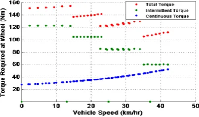
[image:1.595.325.527.605.723.2]

Using real life vehicle parameters [9],[10], wheel torque versus wheel speed curves, as shown in figure, 2 are plotted at zero degree road gradient on IDC. The torque has two components: continuous and intermittent torque, where the continuous torque is required to overcome aerodynamic drag and rolling resistance force and the transient torque is required to overcome inertial forces due to acceleration and grading.

3.

FIELD ORIENTED CONTROL OF

INDUCTION MOTOR (FOC)

A robust induction motor controller has to be designed properly in order to address these frequently varying typical load torque demands at the wheel of the vehicle to run the vehicle efficiently, reliable, safely. In this work authors have proposed indirect field oriented control scheme [11] for the three phase induction motor whose shaft is connected to the wheel of the vehicle through transmission gear arrangement. Here authors have considered 5:1 fixed gear ratio in simulation.

3.1

Principle of IFOC

Author considered d-q model of the induction machine in the reference frame rotating at synchronous speed ωe [7], [8]. The field-oriented control implies that the ids component of the stator current would be aligned with the rotor field and the iqs component would be perpendicular to ids in synchronously rotating reference frame .This was accomplished by choosing ωe as speed of the rotor flux and locking the phase of the reference frame system such that the rotor flux would be aligned precisely with the d axis, as illustrated in Figure below. Now three stator currents were transformed into q and d axes currents in the synchronous reference frames by using the below mentioned transformation in equation 1.

i

e _as

i_{ds 2} cos( ) cos(_{e e} 2 /3) cos( _e 2 /3) i_bs e 3 sin( ) sin( 2 /3) sin( 2 /3)

i_qs e e e

[image:2.595.57.288.421.605.2]

i_cs     _{         }        _{       } _{ }      _{ } (1)

Fig 3: Phasor diagram of FOC

In figure 3, it has been shown that ids and iqs in synchronous reference frame have only dc components in steady state, because the relative speed with respect to that of the rotor filed is zero. The rotor flux-linkages phasor has a speed equal to the sum of the rotor and slip speeds, which is equal to the synchronous speed. Crucial to the implementation of vector control, then, is the acquiring of the instantaneous rotor flux phasor position (θe). This field angle can be written a

e

r

sl

  

(2)

Where,

θ

e is the rotor position and

θ

slis the slip angle. In terms of the speeds and time, the field angle is written as

(

)dt

dt

e

r

sl

e

   

_

 

_

(3)

The field angle was obtained by using rotor position measurement and partial estimation with only machine parameters but not any other variables, such as voltages. Use of this field angle led to a class of control schemes which was known as “Indirect Vector Control” [7], [8].

3.2

Derivation of IFOC

3.2.1

D axes rotor

As for squirrel cage induction motor rotor is short circuited, the rotor d axes voltage equation has been written as

e e e e

V_drR i_{r dr}    p _{dr sl qr} 0 (4)

Where, slip speed

sl

e

r

  

and

e



= speed of rotor

flux vector (synchronous speed) and

r



= speed of rotor. As

r

 is along the d axes of the reference frame so it was

considered that

e

dr

r





and

e

qr



=0, as

r



did not have

any component along q axes due to their orthogonal properties. So, equation 4 has been rewritten as

e

e

R i

_{r dr}

  

p

_dr

0

, here all the variables are referred to stator side.

As e dr

 or

r



constant so after putting this condition we get the following results as

e

p

 

_dr

0

, it implies

_{R i}

e

₀

r dr



and

i

e

dr

=0

3.2.2

Q axes rotor

As for squirrel cage induction motor rotor is short circuited, the rotor d axes voltage equation has been written as

e e e e

V_qrR i_{r qr} p _qr _{sl dr}0 (5)

As e qr

 =0, so the equation 5 has been rewritten as

e e

R i_{r qr} _{sl dr}0

It implies

e (R i_{r qr})

sl _e

dr  



Now e _{L i}e _{L i}e ₀

qr r qr m qs

    and _ie Lm_ie

qr _L qs

r



Again

e

_{L i}

e

_L

_i

e

dr

r dr

m ds

 



as

_i

e

₀

dr



then e _{L i}e

dr m ds

  (6)

Finally, after simplification we got slip speed e i 1 qs sl _e i r _ds     (7)

Where, Lr r _r

r

  is rotor time constant.

3 P e e e e T_e L_m(i_{qs dr}i i_{ds qr}i )

2 2

    (8)

Replacing _ie

dr and ieqr in terms of edr and eqr L

3 P m e e e e

T_e (i_{qs dr} i_{ds qr})

2 2 L_r

      (9)

Putting the condition e qr

 =0, implies that

L

3 P m e e

T (i )

e _{2 2 L} qs dr

r

    (10)

Now if these two currents are controlled then the speed and torque of induction motor will also be controlled.

But these two currents (_ie qs,

e

i_ds) are hypothetical so they have to be transformed into actual currents (_i

a,ib,ic) with the help of

e

 for current control.

cos( ) sin( )

i_{as e e e}

i_ds cos( 2 /3) sin( 2 /3)

i_{bs e e}

e i_qs cos( 2 /3) sin( 2 /3)

i_{cs e e}

      _{ }

   _{ }

      



   _{ }

  _{         }

 

   

 

(11)

3.2.4

Block Diagram Representation

[image:3.595.319.564.114.188.2]

Basic block diagram of the control logic is shown as Figure 4.

Fig 4: Block diagram of Induction Motor drive with IFOC

Speed control of Induction Motor has two loops as shown in the Figure 4.

3.2.5

Outer Speed Loop Control

Outer speed loop is governed by the following mechanical equation:

(12) Where,

ωm which is the mechanical speed, Te is the shaft electromechanical torque, which is control input to the system, TL is the load torque, which is the disturbance input to the system, J & B are plant parameters moment of inertia and coefficient of friction respectively.

Representing the equation in transfer function form,

T (s) T (s) (Js B)_e  _L   _m(s) (13)

So the closed loop system can be represented in the block diagram as shown in figure 5.

Fig 5: Simplified representation of speed controller

[image:3.595.59.289.349.555.2]

3.2.6

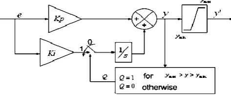
PI Controller with Anti-Windup Scheme

In a normal PI controller, windup is a problem which arises if the input error to the controller is large or remains nonzero for a long time. The output of controller may saturate either because of these reasons which makes the integrator output keep on accumulating. Under this saturation conditions, the controller may give delayed response to any change in the input and this delay would be more if the controller goes into deeper saturation level. So we have to employ anti-windup strategy to prevent the controller from going into deep saturation and to check windup of controller output. To eliminate this, it is necessary to check the integration process during such situations which is in general known as anti-windup [12].

Fig 6: Block diagram representation of a PI controller with anti-windup scheme

The conditional integration method, shown in Figure 4.7, has been adopted by stopping the integration process when the output y has reached the saturation limit. This ensures that while the controller as shown in figure 6 is experiencing saturation there is no further increase in the value of output ‘y’. If the error reduces below certain level for which output comes out of saturation, the integrator starts working again.

3.2.7

Inner current control loop

Hysteresis or Bang-Bang Current Controller: The hysteresis modulation [13], [14] is a feedback current control method where the motor actual current tracks the reference current within a hysteresis band. The controller generates sinusoidal reference current of desired magnitude and frequency which then is compared to the actual motor line current. If current exceeds the upper limit of the hysteresis band, the upper switch of the inverter arm is turned off and the lower switch is turned on. As a result, the current starts to decay. If the current passes the lower limit of the hysteresis band, the lower switch of the inverter arm is turned off and the upper switch is turned on. As a result, the current gets back into the hysteresis band. Hence, the actual current is forced to track the reference current within the hysteresis band as shown in figure 7. d _m

T_e T_L J B _m dt



[image:3.595.320.557.372.469.2]

Fig 7: Principle of Hysteresis Control

4.

SIMULATION RESULTS

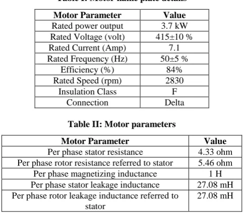
[image:4.595.58.280.72.223.2]

The whole drive train was simulated in MATLAB/SIMULINK where we used the motor parameters and controller parameters as mentioned in Table I to III.

Table I: Motor name plate details

Motor Parameter Value Rated power output 3.7 kW Rated Voltage (volt) 415±10 % Rated Current (Amp) 7.1 Rated Frequency (Hz) 50±5 %

Efficiency (%) 84%

Rated Speed (rpm) 2830 Insulation Class F

Connection Delta

Table II: Motor parameters

Motor Parameter Value Per phase stator resistance 4.33 ohm Per phase rotor resistance referred to stator 5.46 ohm

Per phase magnetizing inductance 1 H Per phase stator leakage inductance 27.08 mH Per phase rotor leakage inductance referred to

stator

[image:4.595.317.558.73.238.2]

27.08 mH

Table III: controller and simulation parameters

Real Time Simulation Parameter Value Kp of Speed Controller 1

Ki of Speed Controller 1 Upper Limit of PI Speed Controller +25 Upper Limit of PI Speed Controller -25 Hysteresis controller band 0.1 Sampling Time (Ts) 1e-4

[image:4.595.318.559.276.433.2]

From figures 8 and 9, it has been observed that the actual speed of the motor is exactly tracking the reference speed of IDC. It ensures that the speed controller is working fine.

Fig 8: Reference speed of Induction Motor (rpm) vs time (sec) in IFOC on IDC with (5:1) gear ratio

Fig 9: Actual speed of Induction Motor (rpm) vs time (sec) in IFOC on IDC with (5:1) gear ratio

[image:4.595.46.289.296.509.2] [image:4.595.317.560.473.667.2]

[image:5.595.56.287.71.248.2]

Fig 11: Zoomed 3 phases actual and reference current (amp) vs time (sec) tracking of Induction Motor in IFOC

on IDC

[image:5.595.318.573.72.229.2]

Figure 10 and 11 depicts the current tracking capability of the current controller in three phases (a,b,c) of the induction motor. There were some amount of ripples in the current but its under limit. It was also observed that during acceleration of the vehicle, current demand by the motor will increase as shown in figure 10 and 11.

Figure 12 depicts the total torque of the motor and load torque at the motor shaft obtained from the vehicle dynamics simulation. Though there were some ripples in the torque profile due to ripples in the current but it was not affecting the speed of the motor. In practical situation due to high inertia, it will not create any problem.

Fig 12: Electromagnetic torque (lower) and load torque (upper) (Nm) vs time (sec) of Induction Motor in IFOC on

IDC

Controller Performance during jerk in sudden bump on road: In figure 13-14, it has been observed that when a 10 Nm load torque was applied for 0.5 sec (jerk) in IDC load torque profile, motor current demand was increased due to high torque requirement but the speed controller and current controller were also working fine under this unwanted situation in the road profile.

[image:5.595.316.574.269.403.2]

Fig 13: Total torque and load torque profile at sudden jerk on road (IDC)

Fig 14: Current Controller performance at sudden jerk on road for 0.5 sec

5.

EXPERIMENTAL RESULTS

The experiments were carried out on the developed test bench as shown in figure 15 using the MATLAB/ Real Time Windows Target platform through Data Acquisition Card (DAQ) between experimental setup and PC to test the functionality of all the power electronic circuits and associated control schemes.

[image:5.595.56.294.431.601.2]

5.1

Speed Controller

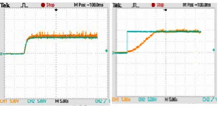
Figure 16 depicts the speed response of the induction motor at 700 and 1000 rpm. It has been observed that actual speed of the induction motor in this control scheme was following the reference speed command. So here outer loop of the proposed control scheme at low speed has been validated.

Figure 16: Speed Tracking (Actual (Yellow) and Reference (Blue) Speed) of Induction motor at 700 rpm and 1000 rpm (X axis: 1div = 5s Y axis: 1 div = 5Volt=500

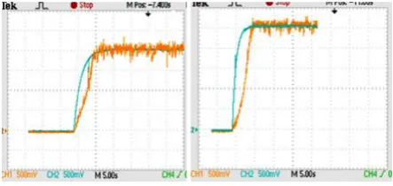
[image:5.595.318.540.593.708.2]

[image:6.595.320.545.71.199.2]

Figure 17 depicts the speed response of the induction motor at 1200, 2000 and 2500 rpm. It has been observed that actual speed of the induction motor in this control scheme was following the reference speed command. So here outer loop of the proposed control scheme at medium speed and high speed has been validated.

Fig 17: Speed Tracking (Actual (Yellow) and Reference (Blue) Speed) of Induction motor at 2000 and 2500rpm (X

[image:6.595.57.279.143.248.2]

axis: 1div = 5s Y axis: 1 div = 500 mV=500 rpm)

[image:6.595.56.276.367.468.2]

Figure 18 depicts the speed tracking accuracy of the controller during arbitrary speed variation between 0 and 800 rpm. It has been observed that actual speed of the induction motor in this control scheme was following the reference speed command. So here outer loop of the proposed control scheme at arbitrary speed variation has been validated.

Fig 18: Speed Tracking (Actual (Yellow) and Reference (Blue) Speed) of Induction motor at 0 to 800 rpm(X axis:

1div = 10s Y axis: 1 div = 2V= 200 rpm)

5.2

Current Controller

Performance of the current controller are shown in figure 19 for the three phases of the induction motor and it has been observed that actual current was tracking the reference current exactly.

Fig 19: a, b, c phases actual (green) and reference (violet) current of the motor at 1000 rpm(X axis: 1div = 10 ms Y

axis: 1 div = 2V =20 amp)

[image:6.595.317.541.369.480.2]

5.3 Performance of the Controller at 1 kW,

2 kW Load:

Figure 20 depicts the controller performance when two and four 500 watt, 250 volt bulb loads were connected across the DC generator. When the motor was rotating at certain speed, DC motor also rotated at that speed and because of the DC motor was operated as DC generator used in this application. It generates voltage which was given to the bulb to glow. It has been also observed that satisfactory speed tracking was occurred when 1 kW and 2 kW resistive loads were connected.

Fig 20: Speed Tracking (Actual (Yellow) and Reference (Blue) Speed) of Induction motor at 1200 rpm at 1 kW load, 1500 rpm at 2 kW load (X axis: 1div = 2.5s,Y axis: 1

div = 500 mV= 500 rpm)

6.

CONCLUSION

In this paper a suitable, robust speed controller for EV has been proposed, and simulated in MATLAB/SIMULINK by taking into consideration of windup phenomenon in PI speed controller at different conditions. A laboratory level experimental setup was developed and no of experiments had been performed to verify the working of circuit topology and control scheme. The results indicate the fulfillment of control objectives. The motor is accelerating and decelerating as per the speed command and the current tracking is satisfactory. From the results it has been concluded that the circuit topology and its control scheme is working fine to cater to the requirements of load torque at the wheel of the vehicle on Indian roads.

7.

REFERENCES

[image:6.595.55.282.582.686.2]

[2] C. C. Chan, The past, present and future of electric vehicle development, in Proc. IEEE 1999 Int. Conf. Power Electronics and Drive Systems, vol. 1, pp. 11– 13,July 1999.

[3] P.Mishra, S.Saha, H.P.Ikkurti, A Methodology for Selection of Optimum Power Rating of Propulsion Motor of Three Wheeled Electric Vehicle on Indian Drive Cycle (IDC), International Journal on Theoretical and

Applied Research in Mechanical

Engineering,Volume2,Issue-1,2013, pp 95-100, ISSN: 2319-3182.

[4] P.Mishra, S.Saha, H.P.Ikkurti, Selection of Propulsion Motor and Suitable Gear Ratio for Driving Electric Vehicle on Indian City Roads, IEEE International Conference on Energy Efficient Technologies for Sustainability (ICEETS’13), pp 692 – 698, April, 2013, ISBN: 978-1-4673-6149-1

[5] G. Nanda, N. C. Kar, A survey and comparison of characteristics of motor drives used in electric vehicles, in Proc. Can. Conf. Electr. Comput. Eng, pp. 811–814, May 2006.

[6] W. Xu and J.G. Zhu, Survey on electrical machines in electrical vehicles, in Proc. Inter. Conf. on Applied Superconductivity and Electromagnetic Devices, Sept. 2009, pp.167-170.

[7] B. K. Bose, Modern Power Electronics and Ac Drives, Prentice Hall PTR, 2002, ISBN0130167436, 9780130167439.

[8] R. Krishnan, “Electric motor drives: Modeling, Analysis, and Control”, Prentice Hall, 2001,ISBN 0130910147, 9780130910141

[9] M Ehsani, Y Gao, S. E. Gay, Ali Emadi, Modern Electric, Hybrid Electric, and Fuel Cell Vehicles: J. Fundamentals, Theory, and Design, CRC press, ISBN: 0-8493-3154-4.

[10]Larminie, J.Lowry, Electric Vehicle Technology Explained, John Wiley & SonsLtd, ISBN-10: 0470851635Dec, 2003.

[11]R. J. Kerkman, T. M. Rowan, and D. Leggate, Indirect Field-Oriented Control of An Induction Motor in The Field Weakened Region, IEEE Trans. Industry Applications, Vol. 28, No. 4,.pp850-857

[12]M. Rehan, A. Ahmed, N. Iqbal, M.S. Nazir, Experimental comparison of different anti- windup schemes for an AC motor speed control system, IEEE, ICET, pp. 342-346, 19-20Oct, 2009.

[13]D. G. Holmes, B. P. McGrath, and S. G. Parker, Current regulation strategies for vector-controlled induction motor drives, IEEE Trans. Ind. Electron., vol. 59, no. 10, pp. 1914–1928, Oct. 2012