Design of Neural Estimator for Non-Linear Interacting
Process
F Fareeza
Research Scholor
Rayalaseema University, Kurnool, Andhra Pradesh, India
B Rama Murthy
, Ph.D Faculty of InstrumentationS.K.University Anantapur, AndhraPradesh, India
ABSTRACT
Real processes often exhibit non-linear behavior; time variance and delay between input and output, having a vast amount of highly correlated data and this correlation need to be utilized in the design of estimator. In this work, an interacting non-linear (conical tank) is taken for study and a neural estimator is designed using Data driven approach. The neural network is developed in hardware on a customized Linux kernel and implemented using python language. The second order training algorithm is modified using a batch update strategy and this approach along with the hardware implementation reduces the estimator training period and makes it highly suited to online.
Keywords
: Non linear process, Non-Interacting system, neural estimator, Back Propagation scheme, Hardware implementation.1. INTRODUCTION
In estimator design, the establishment of a system model is primary and in many cases it is very difficult to obtain the order of stochastic models parsimony Models, especially if the process is highly complex. Even when models are available it is sometimes difficult to propagate the uncertainty through the system dynamics. An alternative framework is to use fuzzy estimator with systems using heuristic knowledge to capture uncertain behavior to build solutions. In this work, an estimator based on fuzzy theory and capable of dealing with random disturbances and “uncertainty” is proposed. Control of conical tank is a challenging problem due to its dynamic cross section. The primary task of a controller is to maintain a process at the desired operating conditions and also to achieve optimum performance in the presence of disturbances. Liquid level control system is an important nonlinear control problem (e.g., the control of level in a conical tank is difficult; as the level decreases). And involves process variable (level), manipulated variable (inflow rate), and load variable outflow rate.
2. LITERATURE SURVEY
The paper represents the application of the partial decoupling control for the nonlinear MIMO hydraulic plant composed of two tanks connected with each other [1]. It designs of the mathematical modeling of tanks conical interacting system process and open loop response of the process obtained. It is not linear- model- based strategy and the control input constraints are directly included in the synthesis [2].A structure of Wiener based nonlinear controller is developed using LabVIEW and implemented in real time. The piecewise response of the system is studied and the gain and time constants for the different regions [3]. A salient feature of the proposed NMPC schemes is that the future trajectory predictions are
based on stochastic simulations, which explicitly account for the uncertainty in predictions arising from the uncertainties in the initial state and the unmeasured disturbances [4].The paper proposed a controller design approach that integrates RTO and MPC for the control of constrained uncertain nonlinear systems. The linearization technique was used to obtain a constant linearization family that is independent of the set point value [5]. In this paper, the static and dynamic robust parametric properties for controlling the liquid level in a single tank was considered as an example of time-varying pseudo linearization of a class of nonlinear systems by input and output (I/O) injection. MITE time-varying linearization up to I/O injection using an injecting or segment function with the single parameter m by a vector description based on the integrator is demonstrated [6]. Several processes are nonlinear and operate under input constraints. They addressed the control of single-input single-output nonlinear systems with input constraints in the presence of modeling errors [7].A nonlinear internal model control based on input output linearization was designed and an internal model control with ant windup which removed the nonlinear mismatch due to input constraints was given [9]. A new model structure selection method was proposed for neural network modelling of non-linear systems. The model structure considered was the NARX model [10]. Proposed a new control scheme of decoupling based decentralized robust control for a typical input two-output system in tandem cold rolling process. A dynamic coupled model of shape and gauge system was developed. Then they proposed new control scheme for combined system [11].In this paper, a systematic approach to design a linear observer to estimate the state vector of a non-linear dynamic system has been presented. The paper represents the method to estimate the state variables, concentration and temperature in the CSTR process [12]. Developed a new intelligent scheme using type-2 fuzzy inference system in neural network structure, with nonlinear system identification and neuro-fuzzy adaptive filter for nonlinear channel equalization [13]
A 550mm T 630mm
250mm 100mm h
10mm
[image:2.595.82.292.77.221.2]V
Fig 1: Conical Tank used for study
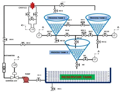
Note: r- radius of the tank, h- Height of the tank The study set up includes non-interacting as well as interacting depending on the valve position. Non-Interacting systems are those systems in which the movement of the final control element of one loop does not affect the process variable of another loop. The
[image:2.595.321.543.131.299.2]non-interacting system is formed by pair of Tank-1 and Tank-3. (Tank-2 inlet closed).The valve settings for interacting & non interacting process are described in Table 1.
Table 1.Valve settings for interacting & non interacting process
Interacting Process
Non- Interacting Process
Hand Valve Setting
MV1, MV4, MV5,
MV7, MV9,
MV10, MV6 and SV1 should be in open condition. MV2, MV11 in partially open condition and other hand valves and solenoid valves in closed condition.
MV1, MV4,
MV5, MV7,
MV9, MV14 and MV13 should be
in open
condition.MV2, MV15 partially open and other hand valves and solenoid valves
in closed
condition.
Fig 2: Process and Instrumentation Diagram
C
S r
r
[image:2.595.110.506.364.666.2]4. NEURAL NETWORK
Neural network involves a large number of processing elements (neurons) working together to solve a specific task. It allows for highly parallel information processing. Neural network is initially fed with large amount of data, which can be used to extract information from complex networks which are not easily noticeable by human or any computer technique.
4.1 NN Training with Back Propagation
The back propagation algorithm is used in layered feed-forward NN to find a local minimum of the error. The algorithm begins training with randomly chosen weights and the goal is to minimize the error by adjusting the chosen weights. The Neural Networks uses the most popular training algorithm such as (i) Enhanced back propagation (EBP) algorithm and (ii) Multi-Layer Perceptron (MLP) network [14]. The constraints to be considered in the NN design are,(i) Larger size
(ii) Poor generalization ability
4.1.1 Design of Estimator
Noise
y x ε(n) E[ε2 (n)]
+ observed
vector Desired vector
Fig3: Design of estimator
Step 1: Set error vector ε(n)
Step 2: Minimize using step 1 and find out weights of the estimator network (done using back propagation algorithm in neural network)
E[ε(n) x.] = 0
Example: If two data vectors x(n) and x(n-1) are observed then E [ε(n) x(n)] = 0
E[ε(n) x(n-1)] = 0
The minimum mean-square error estimation involves conditional expectation which is difficult to obtain numerically. Hence, in this work, the estimation of a parameter tries to optimize some functions of the observed samples with respect to the unknown parameter to be estimated.
The prediction problem addresses the issues of optimal prediction of the future value of the signal on the basis of present and past observations.
4.1.2 Training Data for Neural Network
Input- output data were obtained from the plant and were subsequently used in training the network. Training with back propagation is an iterative process. Back propagation training algorithm is a supervised learning algorithm for multilayer feed forward neural network [17]. The information as to how the mapping was shaped in all regions should be implicitly presented as much as possible in the training data set. The BPN based NN with the inputs FIN FOUT and the output ∆h is shown in Figure 4 where K1, K2&K3 are scaling factors chosen suitably to prevent NN saturation.
B2
W1 W11 W2 W36 B11 Fin W3W6 W37 [0,1] W4
W5 Change in level
W6 W38
Fout [0,1] W7
W8 W39
W9
W35 W40 W10
Fig 4: BPN based NN specifications
4.1.3Problems in Second Order Training
Algorithms (Memory Limitation)
Conventional second order training algorithms are such that, the update formula has the form given in Equation (1),
(JTJ + µI)-1 … (1)
Thus, the size of matrix is proportional to the size of networks and as the size of networks increases, second order algorithms may not be as efficient as the first order algorithms. Practically, the number of training patterns is huge and is encouraged to be as large as possible. In conventional algorithm, the computational duplication exists, i.e.,
(i) Forward computation (calculate errors), and
∑ Estimator ∑ MSE
K1
K2
∑ ∑
∑
∑
∑
∑
∑
∑
∑
∑
(ii) Backward computation: error back-propagation There exists an architectural limitation and also neuron by neuron computation. In second order algorithms, the error back-propagation process has to be repeated for each output. Hence, this is very complex and insufficient for networks with multiple inputs and outputs.
This algorithm works in either of the 2 modes: Incremental mode or batch mode. Usually batch mode is followed due to less time consumption and less no. of propagative iterations. This algorithm is simple to use and well suited to provide a solution to all the complex patterns. Moreover, the implementation of this algorithm is faster and efficient depending upon the amount of input-output data available in the layers. The code flow is given below:
1. Define input – output patterns for training in code
2. Create a network with N input, M hidden, and K output nodes using NN (N, M, K).
3. In class NN,
i. Function __init__ () does the following operations,
It sets the number of input , hidden and output nodes
It activates the nodes.
It creates the weights for input and output nodes using make Matrix (), means number of input and output signals.
It sets the input nodes for random values between (-0.2, 0.2) and output nodes for (0.2,-0.2).
Finally it change the weights for input and output nodes using make Matrix () for momentum.
ii. Function train () does the following operations
This train the code with some pattern, during training with some sample input values, depending on that value it will learn and train itself to get the desired output.
iii. Function update () does the following operations,
Checks whether the input node is equal to length of inputs, if not then raise the error.
It activates the input, hidden and output nodes.
iv. Function back propagate() does the following operations ,
Check whether the output node is equal to length of target; if not then raise the error.
It calculates the error in terms of input and output nodes.
It updates the output and input weights.
This is the function where error correction is done.
v. Function test () does the following operations, Once the code is trained it is required to check whether it has learnt or not, so test is done.
Tests the code with some pattern.
During testing enter the output samples to compare the computed output with the samples
If the computed output does not match the desired output, the difference in the result is back-propagated to the input layer so that the connection weights of the perceptrons are adjusted in order to reduce the error.
The process is continued until the error is reduced to a negligible amount.
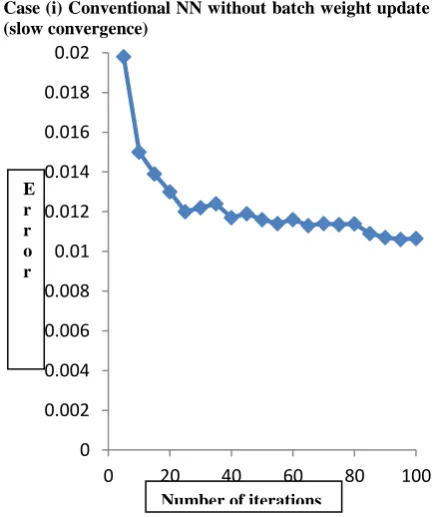
4.2 Trained Network Results
[image:4.595.329.546.188.303.2]Hardware implementation of improved 2nd order computation NN (i.e. proposed BPN trained NN) is implemented in FL2440 Hardware board on Linux kernel using python language is shown in Figure 5. The error plot of conventional and proposed training algorithm is shown in Figure 6.
Fig 5: Hardware Implementation process with Hyper terminal
Case (i) Conventional NN without batch weight update (slow convergence)
Fig 6: Conventional NN error plot
Case (ii) Proposed NN with batch weight update (advantageous)
0 0.002 0.004 0.006 0.008 0.01 0.012 0.014 0.016 0.018 0.02
0 20 40 60 80 100
Number of iterations E
[image:4.595.326.545.347.606.2]Fig 7: Hardware O/P during Training, Test output of Trained NN and error plot for NN (3, 2, 2) (Separable Patterns used for training with
multiple O/P)
Fig 8: Hardware O/P during Training, Test output of Trained NN and error plot for NN (3, 12, 1)
(Inseparable patterns used for training)
5. RESULTS AND DISCUSSION
These results are proven in python language which is experimented in Linux operating system with FL2440 hardware board is updating error during training and tested the trained inputs and given trained neural network output are shown in Figure 9.
(a)
(b)
Fig 9: (a) Error variations during trained (b) Trained NN output
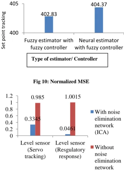
5.1 Performance Metrics
[image:5.595.330.542.157.449.2]The Performance metric results for eliminating level sensor noise (during servo tracking and load variations) are shown in Appendix–I. The normalized MSE values for the estimated level are also shown in Figure10 and Figure 11 respectively.
[image:5.595.84.264.274.424.2]Fig 10: Normalized MSE
Fig 11: Normalized MSE values for the estimated level
6. CONCLUSION
In this paper, neural estimator was designed for a non-linear interacting process. For designing the process, data driven approach was presented. The benefit in fault detection is the ability to directly model a family of fault free system response from the input- output data. The batch update strategy was used to modify the second order training algorithm. Thus, the training period required for the estimator was reduced using the hardware implemented which makes it highly suited for online. The results that were obtained suggest that the designed neural estimator for the non-linear interacting process is effective and further direction of research shall focus on complete hardware implementation integrating the estimator and controller.
7. REFERENCES
[1] Skupin, P., Klopot, W., Klopot, T., “Partially Decoupled DMC System”, International Journal of Systems Applications, Engineering & Development, Issue 3, Vol. 4, 2010.
[2] K. BarrilJawatha, “Adaptive Control Technique for Two Tanks Conical Interacting System”,International Conference on Computing and Control Engineering (ICCCE’12), 12 & 13 April, 2012
-0.9 0.1 1.1 2.1 3.1
0 2 4 6 8 10
E
rr
or
No. of Iterations
-0.4 0.1 0.6 1.1 1.6 2.1
0 1 2 3 4 5 6 7 8 9 10 11 12 13 14 15
Er
ro
r
Number of Iterations
402.83
404.37
400 405
Fuzzy estimator with fuzzy controller
Neural estimator with fuzzy controller
Se
t p
o
in
t
tr
acki
n
g
0.3345
0.0461 0.985 1.0015
0 0.2 0.4 0.6 0.8 1 1.2
Level sensor (Servo tracking)
Level sensor (Resgulatory response)
With noise elimination network (ICA)
Without noise elimination network
[image:5.595.82.297.550.755.2][3] J Satheesh Kumar, P Poongodi and K.Rajasekaran, “Modelling and Implementation ofLabview Based Non-linear PI Controller for a Conical Tank”, Journal of Control & Instrumentation Vol.1, Issue 1, November, pp. 1-9, 2010.
[4] Prakash, J.,Patwardhan,
S.C., Shah,S.L. , “Constrained nonlinear state estimation using ensemble kalman filters”, Industrial and Engineering Chemistry Research, vol. 49, issue 5, pp. 2242 - 2253, 2010
[5] V. Adetola, M. Guay, “Integration of real-time optimization and model predictive control”, Journal of Process Control 20 (2010) 125–133
[6] Static and dynamic robust parameters and PI control tuning of m model for controlling the liquid level in a single tank,SICE Annual Conference 2010, Proceedings of International Conference, 18-21 Aug. 2010, pp. 979 – 984
[7] Q. Hu, P. Saha, G.P. Rangaiah,” Experimental evaluation of an augmented IMC for non linear systems”, Control engineering Practice, Volume 8 (10) Elsevier- Oct 1, 2000,pp. 1167-1176
[8] George Stephanopoulos “chemical process control an introduction to Theory and practice”.
[9] Process Identification from Closed-Loop Response Using Optimization Methods. Viswanathan, P.K.; Rangaiah, G.P. Chemical Engineering Research and Design vol. 78 issue 4 May, 2000. p. 528-541 [10]J.B. Gomm, D.L. Yu and D. Williams, "A new model
structure selection method for non-linear ... 752- 757, Exeter, UK, Institution of Electrical Engineers, 1996
[11]Peng Jing Chaonan Tong ; Lei Xiao “Decoupling Based Decentralized Robust Control for CombinedShape and Gauge System in Tandem Cold RollingProcess” 48th IEEE Conference on Decision andControl and28th Chinese Control ConferenceShanghai, P.R. China, December 16-18, 2009
[12]Prakash, J., Srinivasan, K., “ Non-linear State Estimation for Continuous Stirred Tank Reactor using Neural Network State Filter”,India Conference, 2006 Annual IEEE 15-17 Sept. 2006 Page(s)1 - 4
[13]Ravi, V.R.Thyagarajan, T., “A decentralized PID controller for interacting non linear systems” ,Emerging Trends in Electrical and Computer Technology (ICETECT), 2011 International Conference on 23-24 March 2011Page(s):297 - 302 [14]K.Suresh Manic, R.Sivakumar, V.Nerthiga, R.Akila,
K.Balu, “Design of Plant Estimator Model Using Neural Network”, IJCSNS International Journal of Computer Science and Network Security, VOL.9 No.6, June 2009.
[15]Martin T. Hagan, Howard B. Demuth, Mark Beale, “ Neural Network Design”, China Machine Press, 2002. [16]R. Rojas, “ Neural Networks”, Springer- Verlag,
Berlin, 1996
[17]S.L. Pinjare, Arun Kumar M, “Implementation o Neural Network Back Propagation Training Algorithm on FPGA”, International Journal of Computer Applications (0975-8887) volume 52- No. 6, August 2012.
Appendix-I
Training Data for Neural Network Estimator
Description Eliminating level sensor noise (in Figures)
(a)Fin = 50% Fout=30% Fin – Fout = 20 %,(h +ve)
0 100 200 300 400 500 600
0 200 400 600 800
Time in Seconds
L
e
v
e
l
(b)Fin = 60 %, Fout= 30%, Fin-Fout= 30% (h+ve)
(c)Fin = 60 %, Fout= 80% , Fin-Fout= -20% (h-ve)
(d)Fin = 60 %, Fout= 75% ,
Fin-Fout= -15% (h-ve)
(e) Fin = 60 %, Fout= 65% ,
0 200 400 600 800
0 200 400 600 800
0 100 200 300 400 500 600 700
0 200 400 600 800
0 100 200 300 400 500 600 700
0 200 400 600 800
L
e
v
e
l
in
m
m
Time in Seconds
Time in Seconds
L
e
v
e
l
in
m
m
Time in Seconds
L
e
v
e
l
Fin-Fout= -5% (h-ve)
0 100 200 300 400 500 600 700
0 200 400 600 800