An Empirical Comparison of Data Mining Techniques in Medical Databases

An Empirical Comparison of Data Mining Techniques in

Medical Databases

Kittipol Wisaeng

Mahasarakham University, Mahasarakham,

Thailand.

ABSTRACT

The application of data mining algorithms requires the use of powerful software tools. As the number of available tools continues to grow, the choice of the most suitable tool becomes increasingly difficult. This paper present the basic data mining techniques i.e., naive Bayesian tree, RIpple DOwn Rule, naive Bayes and decision tree algorithm J48 for classifying in medical databases. The goal of this paper is to provide a comprehensive of different classifying techniques in data mining. To evaluate the performance of the above techniques recall, precision and accuracy measures are applied.

General Terms

Data Mining

Keywords

Data mining, naïve Bayesian tree, RIpple DOwn Rule, naïve Bayes, J48

1.

INTRODUCTION

Data mining has a long history, with strong roots in statistics [1], machine learning (ML), database research (BR) and artificial intelligence (AI). Data mining has become a technology in business intelligence (BI) [2], and continues to exhibit steadily increasing importance in technology. Today, a large number of data mining techniques are available such as k-nearest neighbor (KNN) [3], Bayesian networks (BN) [4], case-based reasoning (CBR) fuzzy logic (FL) [5] and genetic algorithms (GA) [6]. As the number of available techniques continues to grow, the choice of the most suitable technique becomes increasingly difficult, each with their own strengths and weaknesses.

In this paper, comparative of data mining techniques for classifying in medical databases namely, naive Bayesian tree, RIpple DOwn Rule, naive Bayes and decision tree algorithm J48 are presented. In this way, we have constructed a large dataset of 4,000 records for an accurate training and testing for our techniques. The techniques following an automated process of knowledge discovery (KDD) i.e., data cleaning, data integration, data selection, data transformation, data mining and knowledge representation. The accuracy of the proposed techniques is evaluated in terms of the percentage of the correctly classified instances from the test data and the difference between values predicted by a model and the values actually observed from the environment that is being modelled. The overall procedure of a comparison data mining techniques is shown in Figure 1.

2.

DATA PREPARATIONS

Sometime, data may be in different formats as it comes from different sources, irrelevant attributes and missing data. Therefore, data needs to be prepared before applying any kind of data mining.

Figure 1. The outline of data mining is the core of KDD in medical databases.

Although at the core of the KDD process [7], this step usually takes only a small part of the overall effort and their details are explained below.

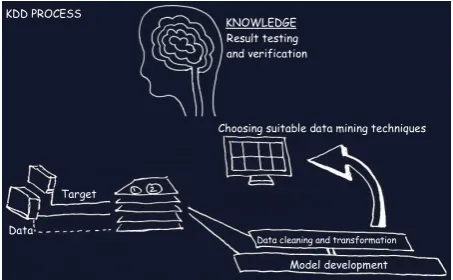
Figure 2.The KDD process of data mining techniques

From Fig.2, the KDD process of data mining techniques is composed of seven main steps: (1) Developing an understanding of the application domain and the goals of the data mining process, (2) Acquiring or selecting a target data set, (3) Data integrating and checking the data set; if the data to be mined comes from several different sources data needs to be integrated which involves removing inconsistencies is name of attributes or attributes values names between data sets of different source, (4) Data cleaning and transformation; this step may involve detecting and correcting errors in the data, (5) Model development; when the data mining

Data Mining Techniques

Automated data Preprocessing

Input Data

Selection

Preprocessing

Transformation

Data Mining

Evaluation

Knowledge

NBT

Ridor

NB

J48

KDD PROCESS

Data Target

Data cleaning and transformation

Model development Choosing suitable data mining techniques

techniques cannot cope with continues attributes, discretization needs to be applied. This step consists of transforming a continuous attribute into categorical attribute, taking only a few discrete values, (6) Choosing suitable data mining technique, and (7) Result testing and verification.

2.1

Data set description

The data sets have different characteristics, such as the number of age from 30 to 89. Also, the characteristics reflect different shapes where some data sets contain a small number of instances. Example of the diabetes mellitus data sets for training and testing purposes as shown in the Table 1, each dataset is described by the data type being used, whether they are categorical, integer or real, the number of instances stored within the data set. Therefore, we use the Min-Max normalization model to transform the attribute’s values to a new range, -1 to 1.

Table 1. Diabetes mellitus data set for training and testing

Attribute Attribute Type Transformed Class

Age Real -0.6798+ Yes/No

Sex Categorical 1 Yes/No

BMI Real, Integer 0.3538+ Yes/No

HT Categorical -1 Yes/No

Genetic Categorical 0 Yes/No

AO Real, Integer 1 Yes/No

Note: BMI, Body Mass Index, HT, Hypertension and AO, abdominal obesity

3.

DATA MINING TECHNIQUES

Data mining techniques can follow three different learning techniques i.e., supervised, unsupervised and semi-supervised [7]. In supervised learning, the technique works with a set of examples whose labels are known. The labels can be nominal values in the case of the classification task, or numerical values in the case of the regression task. In unsupervised learning, in contrast, the labels of the examples in the dataset are unknown, and the technique typically aims at grouping examples according to the similarity of their attribute values, characterizing a classifying task. Finally, semi-supervised learning is usually used when a small subset of labeled examples is available, together with a large number of unlabeled example. Various data mining techniques used for classifying proposed in this paper are explained in the following section.

3.1 Naïve Bayesian Tree

The naive Bayesian tree (NBT) [8], combined naive Bayesian classification and decision tree learning. In an NBT, a local naive Bayes is deployed on each leaf of a traditional decision tree, and an instance is classified using the local naive Bayes on the leaf into which it falls. The formulations of NBT are proposed by [9] and described below.

Algorithm NBT

Input: Π is a set of candidate attributes, and Sis a set of

labeled instances.

Output:A decision treeT.

1. If (Sis pure or empty) or (Πis empty) Return T.

2. ComputePs(ci) on S for each classci.

3. Foreach attributeX in Π, compute IIG(S, X) based on

Eq. (1) and Eq. (2).

4. Use the attributeXmaxwith the highest IIG for the root.

5. PartitionSinto disjoint subsetsSx usingXmax.

6. For all values x ofXmax

6.1 Tx = NT(Π - Xmax, Sx)

6.2 AddTxas a child ofXmax

7. ReturnT.

Before we call the NBT, a set of probabilities P(X|C) should be computed on the entire training data for each attribute and each class. According to the analysis in the preceding section, the total time complexity of the NBT is O(m·n).



x x

S

IG(S, X) = Ent ropy(S) - Ent ropy(S ),

S (1)

where S is a set of training instance, X is an attribute and x is its value, Sx is a subset of S consisting of the instances with

X = x.



i= 1

Ent ropy(S) = - P (c )logP (c ) (2)

where Ps(ci) is estimated by the percentage of instances

belonging to ci in S, and |C| is the number of classes. Entropy

(Sx) is similar.

3.2 RIpple DOwn Rule

Ripple DOwn Rule Learner (Ridor) rule [10] generates a default rule first and then the exceptions for the default rule with the least (weighted) error rate. Then it generates the “best” exceptions for each exception and iterates until pure. Thus it performs a tree-like expansion of exceptions. The exceptions are a set of rules that predict classes other than the default.

Association Rule(R): Implication expressions of the form

X→Y[s, c], whereXandYare item sets. (X, Ysubset ofI)

andX∩Y = empty.

Support(S): Fraction of transactions that contain bothXand

Y. Probability that a transaction containsXUY.

Confidence(C): Measure how often items in Y appear in

transactions that contain X. Conditional probability that a

transaction havingXalso containsY.

3.3 Naïve Bayes

Naïve Bayes (NB) is a simple probabilistic classifier based on applying Bayes’ theorem (or Bayes’s rule) with strong independence (naive) assumptions [11]. The explanation of Bayes rule is defined as Eq. (3).

P (E H)× P (H) P (H E) =

P (E) (3) The basic idea of Bayes’s rule is that the outcome of a hypothesis or an event (H) can be predicted based on some evidences (E) that can be observed. From Bayes’s rule, we have:

1. A priori probability ofHorP(H): This is the probability of

an event before the evidence is observed.

2. A posterior probability of H or P(H|E): This is the

3.4 Decision tree algorithm J48

J48 is slightly modified C4.5 decision tree for classification. The C4.5 algorithm generates a classification decision tree for the give data set by recursive partitioning of data. The decision is grown using depth first strategy (DFS). The algorithm considers all the possible tests that can split the data set and selects a test that gives the best information gain [8]. The formulations of J48 are proposed by [12] and described below. Algorithm J48

Input: T is training data

Output: A decision tree.

1. If (Tbelong to the same categoryC) then Return Nas a

leaf node, and mark it as classC;

2. If attribute is the remainder samples of Tis less than a

give value, then Return Nas a leaf node, and mark it as the

category which appears most frequently in attribute, for each attribute, calculate its information gain ratio.

3. Suppose attribute is the testing attribute of N, the test

attribute equal to the attribute which has the highest information gain ratio in attribute list.

4. If testing attribute is continuous, the find its division

threshold.

5. For each new leaf node grown by nodeN

{

SupposeTis the sample subset corresponding to the leaf

node. If Thas only a decision category, then mark the leaf

node as this category; else continue to implement J48-Tree

}

6. Compute the classification error rate of each node, and

then prune the tree.

4. PERFORMANCE EVALUATION

The algorithms performance was assessed using the recall, precision and accuracy on test set. Recall is the fraction of relevant instances that are retrieved (TP/TP+FN). Precision is the fraction of retrieved instances that are relevant (TP/TP+FP). Accuracy is the overall success rate of the algorithms (TP+TN/TP+FP+FN+TN). All measures can be calculated based on four values [13], namely True Positive (TP, is a number of correctly predictions that an instances positive), False Positive (FP, is a number of incorrect predictions that an instance is positive), False Negative (FN, is the number of incorrect of predictions that an instance negative), and True Negative (TN, is the number of correct predictions that an instance is negative). These values are defined in Table 2.

Table 2. Confusion Matrix.

Predicted Class

True class Yes No Total

Yes TP FN TP+FN

No FP TN FP+TN

Total TP+FP FN+TN TP+FN+FP+TN

5. EXPERIMENTAL RESULTS

The experimental results under the framework of Waikato Environment for Knowledge Analysis (WEKA; version 3.6.10) [14]. All experiments were performed on a Duo Core with 1.8GHz CPU and 2G RAM. We have performed of several data mining techniques to select the one with the most accurate results to use in medical data set. We choose four very commonly used techniques namely, NBT, Ridor, NB and J8. To have a fair comparison between different techniques, training time in seconds and tree size ratio for each technique on each data set obtained via 10-fold stratified cross validation.

5.1 Results for classification using NBT

NBT is applied on the data set and the confusion matrix is generated for class gender having two possible values (Yes/No).

NBTree

---BMI <= -0.8: NB 1

BMI > -0.8

| BMI <= 0

| | Sex <= 0

| | | GE <= 0: NB 5

| | | GE> 0: NB 6

| | Sex > 0: NB 7

| BMI > 0: NB 8

Number of Leavesis 5 and Size of the tree is 9. Time taken to build model is

0.89 seconds

--- Confusion Matrix---

a b <-- classified asinstances: 4000

880 0 | a = Yes

0 3120 | b = No

---For above confusion matrix [15], TP for class a (Yes) is 800 while FP is 0 whereas, for class b (No), TP is 3120 and FP is 0 (diagonal element of matrix 880+3120 = 4000 represents the correct instances classified and other elements 0+3120 = 3120 represents the incorrect instances). Therefore, TP rate equals diagonal element divided by sum of relevant row, while FP rate equals non-diagonal element divided by sum of relevant row (TP rate for class a = 880/(880+0) = 0, FP rate for class a = 0/(0+3120) = 0, TP rate for class b = 3120/(0+3120) = 1, and FN rate for class b = 0/(880+0) = 0).

5.2 Results for classification using Ridor

Ridor is applied on the data set and it generates a default rule first and then the exceptions for the default rule with the least (weighted) error rate. Then it generates the "best" exceptions for each exception and iterates until pure.

Ridorrules

---Target = Yes (4000.0/3120.0)

Except(BMI>0) and (AGE>-0.790698) => Target = No(1229.0/0.0) [611.0/0.0]

Except (AGE>0.465117) => Target = No (691.0/0.0) [349.0/0.0]

Except (BMI>0.4) => Target = No (48.0/0.0) [32.0/0.0]

Except (GE> 0) and (BMI>-0.8) and (HT<= 0) and (AGE>-0.651163)

=> Target = No (107.0/0.0) [53.0/0.0]

Total number of rules (incl. the default rule is 5 and time taken to build model

is 0.11 seconds.

--- Confusion Matrix---

a b <-- classified asinstances: 4000

832 48 | a = Yes 26 3094 | b = No

---

For above confusion matrix, TP for class a (Yes) is 832 while FP is 48 whereas, for class b (No), TP is 3094 and FP is 26 (diagonal element of matrix 832+3094 = 3926 represents the correct instances classified and other elements 480+26 = 506 represents the incorrect instances). Therefore, TP rate equals diagonal element divided by sum of relevant row, while FP rate equals non-diagonal element divided by sum of relevant row (TP rate for class a = 832/(832+48) = 0.94+, FP rate for class a = 26/(26+3094) = 0.008+, TP rate for class b = 3094/(26+3094) = 0.99+, and FN rate for class b = 48/(832+48) = 0.05+).

5.3 Results for classification using NB

Class for a NB classifier using estimator classes. Numeric estimator precision values are chosen based on analysis of the training data. For this reason, the classifier is not an updateable classifier (which in typical usage are initialized with zero training instances), if you need the updateable classifier functionality, use the NB updateable classifier. The NB updateable classifier will use a default precision of 0.1 for numeric attributes when build classifier is called with zero training instances.

Naive Bayes Classifier

---

Class: Yes No Attribute (0.22) (0.78)

---

Sex mean 0 0 std. dev. 0.3333 0.3333 weight sum 880 3120 precision 2 2

BMI

mean -0.4 0.0103 std. dev. 0.3411 0.2307 weight sum 880 3120 precision 0.4 0.4

GE mean 0 0 std. dev. 0.3333 0.3333 weight sum 880 3120 precision 2 2 AGE

mean -0.404 0.1083 std. dev. 0.362 0.6462 weight sum 880 3120 precision 0.0741 0.0741

HT mean 0 0 std. dev. 0.3333 0.3333 weight sum 880 3120 precision 2 2

AO

mean 0 0 std. dev. 0.3333 0.3333 weight sum 880 3120

precision 2 2

Time taken to build model is 0.02 seconds ---Confusion Matrix---

a b <-- classified asinstances: 4000

400 480 | a = Yes 80 3040 | b = No

---

For above confusion matrix, TP for class a (Yes) is 400 while FP is 480 whereas, for class b (No), TP is 3040 and FP is 80 (diagonal element of matrix 400+3040 = 3440 represents the correct instances classified and other elements 480+80 = 560 represents the incorrect instances). Therefore, TP rate equals diagonal element divided by sum of relevant row, while FP rate equals non-diagonal element divided by sum of relevant row (TP rate for class a = 400/(400+480) = 0.45+, FP rate for class a = 80/(80+3040) = 0.25+, TP rate for class b = 3040/ (80+3040) = 0.97+, and FN rate for class b = 480/(400+480) = 0.54+).

5.4 Results for classification using J48

J48 is applied on the data set and the confusion matrix is generated for class gender having two possible values (Yes/No). Class for generating a pruned or unpruned C4.5 decision tree[16].

J48 tree

---

BMI <= -1: Yes (320.0)

BMI > -1

| AGE <= 0.395349

| | BMI <= -0.2

| | | HT <= -1

| | | | GE <= -1: Yes (80.0)

| | | | GE > -1

| | | | | AGE <= -0.674419: Yes (80.0)

| | | | | AGE > -0.674419: No (160.0)

| | | HT > -1: Yes (320.0)

| | BMI > -0.2

| | | AGE <= -0.813953

| | | | Sex <= -1: No (80.0)

| | | | Sex > -1: Yes (80.0)

| | | AGE > -0.813953: No (1360.0)

| AGE > 0.395349: No (1520.0)

Number of Leaves is 9, size of the tree is 17 and time taken to build model: 0.11

seconds.

---Confusion Matrix---

a b <-- classified asinstances: 4000

866 14 | a = Yes 21 3099 | b = No

---

For above confusion matrix, TP for class a (Yes) is 866 while FP is 14 whereas, for class b (No), TP is 3099 and FP is 21 (diagonal element of matrix 866+3099 = 3965 represents the correct instances classified and other elements 14+21= 35 represents the incorrect instances). Therefore, TP rate equals diagonal element divided by sum of relevant row, while FP rate equals non-diagonal element divided by sum of relevant row (TP rate for class a = 866/(866+14) = 0.98+, FP rate for class a = 21/(21+3099) = 0.006+, TP rate for class b = 3099 (21+3099) = 0.99+, and FN rate for class b = 14/(866+14) = 0.01+).

5.5 Results analysis

results of the NBT, Ridor, NB and J48 techniques. All the experiment results are shown in Table 3.

Table 3. Diabetes mellitus data set for training and testing

Parameter Data mining techniques

NBT J48 Ridor NB

Recall 1.0 0.98+ 0.94+ 0.86

Precision 1.0 0.99+ 0.99+ 0.85+

Accuracy 100 99.1+ 98.1+ 86.00

MAE 0.003 0.004 0.005 0.18+

RMAE 0.01+ 0.02+ 0.03+ 0.31+

Time (second) 0.09 0.11 0.1 0.02

Note: Accuracy value as percentage (%).

Table 3, shows the performance of for data mining techniques based on recall, precision, accuracy, mean absolute error (MAE), root mean absolute error (RMAE) and time taken to build each model for the individual techniques, respectively. From Table3, the rank of accuracy for these data mining techniques is NBT (100%), J48 (99.1%), Ridor (98.1%), and NB (86%). Of all the data mining techniques, NB has highest speed in building the model and takes 0.02s while J48 is the slowest model requiring 0.11s for the same data set. Considering both accuracy and speed, NBT technique are the best choices.

6. CONCLUSIONS

This paper has conducted a comparison between four data mining techniques namely, NBT, Ridor, NB and J48 relies on the careful KDD steps could be used to classification in medical databases. The performance of the techniques is validated by recall, precision and accuracy values. The NBT technique show better performance for our medical databases (100%), but J48 and Ridor are also useful and may be better fit to deal with our case.

In the process of KDD, choice of parameters and the construction of high quality training and test data sets are important steps.

Overall, our experimental results show that careful KDD steps and appropriate technique together provide best classification in medical databases This technique intends to help expert in risk factor analysis in diabetes mellitus to faster and more easily.

7. ACKNOWLEDGMENTS

This paper was supported by the Mahasakham Business School, Mahasahakham University. We also would like to thank Mahasarakham Hospital for the medical databases used in this experiment.

8. REFERENCES

[1] Mikut, R., Reischl, M. 2011. Data mining and knowledge

discovery, Wiley Interdisciplinary Reviews, pp.431-443.

[2] Barrett, T., Troup, D., Wilhite, S., Ledoux, P., Rudnev, D., Evangelista, C., Kim, I., Soboleva, A., Tomashevsky, M., Edgar, R. 2007. NCBI GEO: Mining tens of millions of expression profiles-database and tools update, Nucleic Acids Re., pp.760-765.

[3] Cover, T., Hart, P. 1967. Nearest neighbor pattern classification, IEEE Transactions on Information Theory, pp.21–27.

[4] Darwiche, A. 2009. Modeling and reasoning with

Bayesian networks, Cambridge University Press, pp. 1-562.

[5] Castro, J.R., Castillo, O., Martinez, L.G. 2007. Interval Type-2 Fuzzy Logic Toolbox, Engineering Letters, pp. 89-98.

[6] Minaei-Bidgoli, B., Punch, W. 2003. Using genetic

algorithms for data mining optimization in an educational

web-based system, Genetic and Evolutionary

Computation, pp: 2252-2263.

[7] Sunita, B., Jitender, A. 2012. Classification and feature selection techniques in data mining, International Journal of Engineering Research & Technology, pp. 1-6.

[8] Yongheng, Z., Yanxia, Z. 2007. Comparison of decision

tree methods for finding active object, Advances of Space Research, pp. 1955-1959.

[9] Jiang, S., Harry, Z. 2006. A fast decision tree learning algorithm, In Proc. of the National Conference on

Artificial Intelligence, American Association for

Artificial Intelligence, pp. 1-6.

[10]Datta, R.P., Sanjib, S. 2011. An empirical comparison of rule based classification techniques in medical databases, Working Paper, Indian Institute of Foreign Trade, pp. 1-18.

[11]Choochart, H. 2008. A tutorial on naïve Bayes

classification, pp. 1-6.

[12]Yogendra, K.J., Upendra. 2012. An efficient intrusion detection based on decision tree classifier using feature reduction, International Journal of Scientific and Research Publications, pp. 1-6.

[13]Samuel, A.M., Daniel, M.D., James, K., Gray, M.W. 2009. Are decision trees always greener on the open (source) side of the fence?, In Proc. of the Inter. Conf. on Data Mining. pp. 185–188.

[14]Hall, J., Frank, E., Holmes, G., Pfahringer, B., Reutemann, P., Witten, I. 2009. The WEKA data mining software: an update, ACM SIGKDD Explorations Newsletter, pp. 10-18.

[15]Tina, R.P., Sherekar, S.S. 2013. Performance analysis of naïve Bayes and J48 classification algorithm for data classification, Inter. Jour. of Computer Science and Applications, pp. 256-261.