1
Effect of Hypersonic Flow Physics Modeling on
Electro-Optical Sensor Assessment
Lauren E. Mackey1 and Iain D. Boyd2
Department of Aerospace Engineering, University of Michigan, Ann Arbor, MI 48109
Timothy Leger3, Ryan Gosse4,and Konstantinos Vogiatzis5
U.S. Air Force Research Laboratory, Wright-Patterson Air Force Base, OH 45433
A potential future use of hypersonic platforms is for Intelligence, Surveillance, and Reconnaissance (ISR). It is common for these types of missions to employ electro-optical sensors to collect information. The type of high-speed flow analysis needed to perform reliable assessments of the performance of electro-optical sensors is unclear. In the present study, numerical simulations are utilized to perform flow calculations at varying levels of modeling fidelity. The simulations are performed at Mach 11 on a hemisphere flare and at Mach 6 on a flat plate. The hemisphere flare cases are used to determine the effects of including real-gas thermochemical non-equilibrium modeling. For these studies, the more computationally expensive method of accounting for thermochemical non-equilibrium produces optical path differences (OPDs) that are less than 100% larger. The flat plate test cases are performed using air as a perfect gas with varying levels of turbulence modeling and resolution. The cases are run using a laminar flow assumption (no turbulence), the Menter SST closure model for the Reynolds Averaged Navier-Stokes equations, and implicit large eddy simulation (ILES). The OPDs produced by ILES can be as much as two orders of magnitude larger than solutions produced by the Menter SST model and laminar flow.
Nomenclature
OPD = Optical Path Difference [m]OPL = Optical Path Length [m]
t = Time [s]
X = Mass Fraction
τ = Shear Stress
u = Velocity [m/s]
e = Energy [kg m2/s2]
q = Heat Transfer [W/m2] 𝜔̇ = Source Terms 𝜏𝑟 = Relaxation Time [s]
𝜏𝑟𝑘 = Interspecies Relaxation Time [s]
M = Mach Number
n = Index of refraction
T = Temperature [K] p = Pressure [kPa]
ρ = Density [kg/m3]
KGD = Gladstone-Dale constant
l = Coordinate along line of sight [m]
Downloaded by UNIVERSITY OF MICHIGAN on April 5, 2018 | http://arc.aiaa.org | DOI: 10.2514/6.2017-3836
48th AIAA Plasmadynamics and Lasers Conference 5-9 June 2017, Denver, Colorado
Subscripts
∞ = Freestream
s = Species
i = Index
j = Index
* = Equilibrium <> = Mean
I. Introduction
S
technology advances, flight in the hypersonic regime is becoming more attainable. The new technology will allow vehicles engaged in intelligence, surveillance, and reconnaissance (ISR) missions to travel in high speed conditions. If hypersonic ISR vehicles are to be developed, differing flowfield effects (from lower speed flows) may need to be considered or emphasized to accurately assess signal propagation through the media around the vehicle. Most ISR vehicles have operated in the sub or supersonic regimes, where the physical flow acts very differently from high speed, high enthalpy flows. Studies need to be conducted on optical propagation in hypersonic flows because existing methods of analyzing optical sensing may not produce accurate results for high speed flows, or the lower speed methods may be very costly at high Reynolds numbers.A hypersonic environment is a harsh environment where conditions could potentially obscure the signals used by optical sensors to a larger extent than in lower speed flows. The high speed flow effects that need to be considered are strong shocks and high aerodynamic heating. These phenomena result in thermochemical non-equilibrium. Non-equilibrium regions are characterized by molecules that are reaching or have reached excited states. These molecules often have vibrational and translational temperatures that are not equal. Non-equilibrium flow is also characterized by chemical species that are dissociating in areas of high temperatures and then potentially recombining near the vehicle’s cooler surface. These effects need to be understood and may need to be included in the performance of optical calculations in the hypersonic regime. As an optical beam traverses a non-equilibrium flow field, it will encounter varying densities of the dissociated and undissociated species. Each of these atoms or molecules has distinct optical properties that may need to be accounted for in performing optical calculations.
Considering turbulent effects is also be integral to the assessment of the flowfield surrounding the ISR vehicle. The length scales and speeds of these vehicles often dictate that the simulations must be treated as occurring in the turbulent regime. Turbulence is characterized by fluctuations in the bulk flow quantities. Density influences the optical characteristics of the flow, as can be seen in the Gladstone-Dale relation, and fluctuations in optical characteristics distort the beam as it traverses the field surrounding the ISR vehicle.1
While many studies have shown the importance of including well resolved turbulence in aero-optical calculations, these studies are often conducted on thicker, lower Reynolds number boundary layers.2 At high Reynolds numbers, the inertial forces have greater significance which can promote thinner boundary layers; this could minimize the effects of turbulence in the flow. These studies also do not often present various methods of obtaining turbulence flow data and weigh the added cost of additional turbulence resolution against the information gained in terms of optical calculations.
Few studies use the results of thermochemical non-equilibrium simulations to calculate the optical properties of a beam as it travels through various flow configurations.2 Most optical studies use only low enthalpy perfect gas flows. The published data also reflect the consideration of only perfect air as the mixture for calculating the optical properties, e.g. index of refraction.2 The media surrounding a hypersonic vehicle cannot always be accurately represented by a perfect gas. It is not immediately apparent, however, the extent to which including these effects will affect the optical distortions.
In the present study, two separate sub-investigations are performed. The first involves studying an optical beam as it travels through a Mach 11.2 flow around a hemisphere-flare. Laminar simulations are conducted using perfect gas and real gas models in 5 species air (N2, O2, NO, N, O). The hemisphere-flare test case is designed to induce non-equilibrium effects. This study makes it possible to determine the effects of including non-equilibrium on beam propagation evaluations. Thus, it will be possible to determine whether incurring the extra cost associated with non-equilibrium calculations is necessary or if the lower cost perfect gas simulations lead to similar optical results. This study assumes the non-equilibrium real gas simulation provides the more accurate description of the flow field.
A
The hemisphere flare simulation presented in this paper focuses on boundary layer flow and includes modeling the effects of non-equilibrium through the use of Park’s model for the effects of vibrational non-equilibrium on chemical reactions and the Landau-Teller model for vibrational relaxation.
The second sub-investigation involves Mach 6 flows over a flat plate. These tests are performed using implicit large eddy simulation (ILES), the Menter SST closure to the Reynolds averaged Navier-Stokes (RANS) equations, and laminar flow solutions. This set of tests makes it possible to quantitatively compare the varying levels of turbulence resolution. In this type of flow, non-equilibrium effects are unimportant and are not included. From the flat plate data, it can be determined whether costs associated with running an ILES simulation are necessary or if the solution provided by, for example, a RANS solution, is acceptable. This study assumes ILES provides the more accurate description of the flow field.
The optical calculations are carried out as a post processing step for both geometries. A separate grid is created for the optical calculations and the appropriate integrations are conducted along the signal propagation path.
This paper first presents the numerical methods employed for the mean flow and the optical calculations. The simulation setup and results are split into two sections; one describes the effects of including non-equilibrium modeling on optical calculations and the other, the effects of including various level of turbulence resolution on optical calculations. The final section of the paper discusses the differences in optical calculation results.
II. Numerical Approach
The numerical method can be separated into two steps. The first step involves simulating the flow around the vehicle of interest. The second step involves performing the optical calculations.
A. Flow Field Calculations
The non-equilibrium study and the turbulent study’s laminar and Menter SST flowfield calculations are conducted using the University of Michigan’s hypersonic computational fluid dynamics (CFD) code LeMANS.3 LeMANS can solve for turbulent, high enthalpy flows that experience thermochemical non-equilibrium. LeMANS assumes that the flow is in the continuum or near continuum regime.This code couples the Navier-Stokes equations with thermodynamic and transport property models.3 Also included in the code are models for finite rate chemistry and energy relaxation models.3 LeMANS works by taking the Navier-Stokes equations and integrating these equations spatially and temporally. To integrate spatially, the finite volume method is implemented. Fluxes across each cell are calculated using a flux vector splitting scheme for the inviscid components and a central scheme for the viscous parameters.3 LeMANS assumes that the fluid is Newtonian, and thus the shear stress can be calculated using Stokes’ hypothesis.LeMANS is second-order accurate in space and time. For closure in turbulence modeling, LeMANS uses the Menter SST, the Menter BSL, or the Spalart-Allmaras closure models.4,5 The Menter SST model is chosen in this study for its ability to solve for near-wall regions.
The ILES in this study is conducted using the finite volume US3D code, a high speed computational fluid dynamics code that was created by the University of Minnesota.6 US3D can also couple the Navier-Stokes equations with thermodynamic and transport property models. US3D, like LeMANS, couples the mean flow equations with finite rate chemistry and energy relaxation models; however, it should be noted that the non-equilibrium features of US3D are not utilized in this study. 6 This code is used only for the perfect gas implicit large eddy simulation. The viscous terms are calculated using a 2nd order central scheme. The inviscid terms are calculated using a sixth order scheme. 6 Low dissipation schemes are what allow for turbulence calculations to be conducted. There are many second order LES codes. High order helps in reducing the number of grid points required to resolve the turbulence. The US3D turbulence simulation uses an implicit filter. An implicit LES does not resolve the smallest flow features. Instead, it relies on the grid to act as the filter. All features that are not resolved will be dissipated. This is acceptable for an optical study because the most optically important turbulent features in boundary layer flow are approximately the size of the boundary layer.2 Turbulence on the flat plate is created by imposing alternating pairs of counter-rotating vortices in a laminar boundary layer profile at an inflow plane at x=0.0375 meters. These vortices create both down and up-wash flow features, which quickly induce type 1 transition and result in a turbulent boundary layer.6 It should be noted that the laminar and Menter SST simulations were adjusted for the initial laminar boundary layer thickness
species equation are found using standard finite rate chemistry. The effects of thermal non-equilibrium on the reaction rates are accounted for using Park’s two temperature model.7
The vibrational energy transport equation is solved with the aid of the Lumped Landau-Teller Relaxation (LLTR) approximation, which is as follows:8
𝑄 = ∑ 𝜌
𝑠(𝑒
𝑣∗𝑠− 𝑒
𝑣𝑠)
𝜏
𝑟 𝑠(1)
where Q energy exchange rate between vibrational and translational energy modes, 𝑒𝑣𝑠
∗ is the vibrational energy of
species s at the local translational energy if the flow were in equilibrium and 𝑒𝑣𝑠 is the vibrational energy of each species. The relaxation time is found using the following expression:3
𝜏
𝑟=
∑ 𝑋
𝑟 𝑟∑ 𝑋
𝑟 𝑟/𝜏
𝑟𝑠(2)
The interspecies relaxation time,𝜏𝑟𝑠, is found using the Millikan and White approximation.9 For simplicity, the
vibrational energy of each molecule is treated as a harmonic oscillator. The source term for the vibrational energy equation is then found by adding Q (eqn.1) to the vibrational energy produced by chemical reactions.
B. Optical Assessments
Optical assessment of an initially planar wave front begins with obtaining the index of refraction of the medium i.e., the air around the vehicle. The index of refraction can be found from the density profile using the Gladstone-Dale relation as follows:1
𝑛 = 𝐾
𝐺𝐷𝜌 + 1 (3)
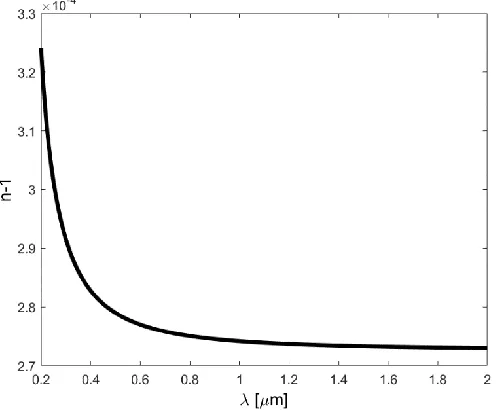
[image:4.612.179.427.467.672.2]where n is the index of refraction, ρ is density and KGD is the Gladstone-Dale constant. In the perfect gas simulations only one Gladstone-Dale constant is used (2.27 x10⁻⁴ m3/kg). As can be seen in Fig.1, which shows index of refraction as a function of wavelength, the index of refraction, and consequently the Gladstone-Dale constant, is nearly constant when near the visible spectrum or when 0.7µm > λ > 0.5µm.10 This suggests that the Gladstone-Dale constants are applicable to all wavelengths greater than 0.5 µm.
Figure 1. Index of refraction as a function of wavelength
In the real gas simulations, the effects of dissociation are also included, and thus the Gladstone-Dale constant is modified in the following manner:11,12
𝐾
𝐺𝐷= ∑ 𝐾
𝑠(
𝜌
𝑠𝜌
) (4)
where Ks is the Gladstone-Dale constant for each species, ρs is the species density, and ρ is the total density. For the real gas simulation, the Gladstone-Dale constants are 2.40 x10⁻⁴ m3/kg,3.10 x10-4 m3/kg, 1.93 x10⁻⁴ m3/kg,2.04 x10-4 m3/kg,2.21 x10-4 m3/kg,for N2, N, O2, O, and NO respectively.11,12,17 All of these values were experimentally obtained at wavelengths of approximately 0.5 µm. It should be noted that the entire temperature and pressure range that these constants are useful is unknown. It has been suggested that these constants may not change precipitously with temperature.11
Once the index of refraction is known, it is then possible to find the optical path length (OPL). This value is the product of the geometric distance a wave travels and the index of refraction. It can be thought of as the distance a wave front would travel in a vacuum in the same time it takes the wave front to traverse the geometric distance of interest.13 When the index of refraction varies, as it does in this study, OPL is found as follows:
𝑂𝑃𝐿 = ∫ 𝑛(𝑙)𝑑𝑙 (5)
Often of more interest in considering optical aberrations is the difference in optical path length between a portion of the wave front and a reference value, usually taken to be the spatially averaged OPL. This difference is referred to as optical path difference (OPD) and is found using the following equation:
𝑂𝑃𝐷 = 𝑂𝑃𝐿− < 𝑂𝑃𝐿 > (6)
OPD indicates how much the OPL varies from the mean value across the sensor aperture.13
The integral in Eq. (5) is solved by creating a mesh for the optical calculations that has cells approximately equal in size to those of the CFD mesh; however, the optical mesh is aligned with the direction of signal propagation. For this study the beams radiate outwards from the wall boundary. The density from the fluid simulation is linearly interpolated onto the optical mesh. The path of the signal propagation is integrated along to obtain the total OPL. The spatially average OPL is subtracted and the result is the OPD. The current method for calculating optical aberrations is not tightly coupled to the flow field calculations; either a steady-state flow solution is used (for the laminar and Menter SST simulation), or solutions at specific times (for ILES) are used.
III. Simulation Parameters
The simulation set-up can be arranged into two sections. The first subsection describes the simulations that are used to discern the effects of including thermochemical non-equilibrium models in aero-optical assessments. The second subsection details the simulations that are used to compare various levels of turbulence resolution on the optical calculations.
A. Non-Equilibrium Study
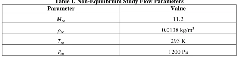
The non-equilibrium portion of this study is conducted on a 2D axisymmetric body that has a nose radius of 7 mm; see Fig. 2 for illustration. This case is designed to include non-equilibrium effects. The 5 species air freestream flow conditions are shown in Table 1.
Table 1. Non-Equilibrium Study Flow Parameters
Parameter Value
𝑀∞ 11.2
𝜌∞ 0.0138 kg/m3
𝑇∞ 293 K
𝑃∞ 1200 Pa
These values correspond to a Reynolds number of 3.5 x10⁶ m-1. It should be noted that an isothermal wall boundary condition is used with a wall temperature of 1000 K. The wall is non-catalytic.
The non-equilibrium flowfield simulations are run on a fully converged 130 (body direction) nodes x 90 (normal direction) nodes mesh. The cells adjacent to the wall have a Reynolds number of one and are then stretched as the freestream is approached. The two simulations run on this mesh are as follows: laminar real gas and laminar perfect gas. A basic grid convergence study is conducted where finer meshes are used until the solutions cease to change. Three meshes are tried for each simulation. The computational time for the perfect gas simulation is approximately 34 CPU hours, while the computational time for the real gas simulation is approximately 42 CPU hours. For completeness the perfect and real gas cases are also run with the Menter SST closure model. A new mesh was created to insure that the y+; a distance from the wall that is nondimensionalized with friction velocity, viscosity, and density; in the cell adjacent to the wall is 1. The fully converged mesh the turbulent simulations are run on is 130 (body direction) nodes x 110 (normal direction) nodes. The turbulent perfect gas simulation takes approximately 62 CPU hours to converge, and the turbulent real gas simulation takes approximately 80 CPU hours to converge.
B. Turbulence Study
[image:6.612.113.498.420.509.2]The simulations that are used for determining the effects of various levels of turbulence modeling/resolution are conducted on flow over a flat plate. The flat plate length for all simulations is 0.5625 meters. For the ILES case the length in the z dimension in 0.1475 meters. This case is run assuming a perfect gas in order to isolate the effects of the varying turbulence approaches; see Table 2 for the perfect air freestream conditions.
Table 2.Turbulence Study Flow Parameters
Parameter Value
𝑀∞ 5.74
𝜌∞ 0.144 kg/m3
𝑇∞ 274 K
𝑃∞ 11300 Pa
The unit Reynolds number for these simulations is 1.7 x10⁷ m-1. The isothermal wall is set to 300 K. The laminar and Menter SST solutions are run on fully converged meshes. As with the non-equilibrium study, the simulations are run on various meshes until the solution ceases to change. The ILES mesh is created to have ∆x+ = 27.38, a ∆z+ = 32.8, and a ∆y+ = 0.2. These values are sufficient for an ILES simulation.14
Table 3. Computational Time for Turbulent Simulations
Simulation Mesh Computational Time
Laminar 100 x 64 1.93 hours
Menter SST 119 x 100 2.47 hours
ILES 5389 x 296 x 181 864,000 hours
The size of all meshes is described in nodal dimensions, not numbers of cells. The mesh for the laminar study has a Reynolds number of one in the cells adjacent to the wall. Another mesh is created for the Menter SST simulation; it is created to ensure that the y+ is at most one in the cells adjacent to the wall. For both the laminar and the Menter
SST simulations, meshes were created in two dimensions. In contrast, the ILES mesh is three-dimensional to obtain physical results. Turbulence is a three dimensional phenomenon and the detailed ILES modeling requires simulations to be performed in full three dimensions. For ILES, the mesh is divided horizontally into three regions. The first consists of a y+ of 0.2 at the wall stretching to a y+ of 20. The second region has equal spacing and extends to point at which 1.4 times the expected boundary layer at the exit plane is reached. The third region is then stretched to the top boundary.
IV. Results
As in the simulation description, the results of this study are separated into two sections. The first subsection presents the results involving the inclusion of non-equilibrium models, and the second subsection presents the results of including various levels of turbulence modeling fidelity
.
A. Effects of Thermochemical Non-Equilibrium
[image:7.612.162.428.287.520.2]As can be seen in Fig. 2, the flow consists of a strong shock surrounding the body. Figure 2 illustrates the differences between the flow of a real gas and a perfect gas.
Figure 2. Temperature contours obtained from real gas and perfect gas laminar simulations for the Mach 11 hemisphere flow
The maximum temperature reached in both simulations is 7000 K, which imparts enough energy for the molecules in air to begin to dissociate. For the non-equilibrium simulations, energy goes into breaking the bonds of the diatomic molecules; this explains the lower near wall temperatures in the real gas simulations. The flow has a thin boundary layer near the wall, typical of high-speed flows. Figure 3 shows the densities of the dissociated species in the non-equilibrium simulation at one y location in Zone A and one x location in Zone B; see Fig. 2 for Zone definitions. The data for both zones is extracted normal to the surface.
Perfect Gas
Real Gas
A
B
Figure 3. Species Densities for (A.) Zone A and (B.) Zone B
As Fig. 3 shows, the dissociated species are significant, especially near the wall; the density of NO and O are on the same order of magnitude as N2 and O2.
The optical calculations are carried out in the two zones, denoted as A and B in Fig. 2. These zones were chosen because they are locations were sensors could potentially be located and they experience quite different flow phenomena. For example, flow in Zone A will experience a strong shock and high heating while flow in Zone B experiences a weaker shock. Total density curves are extracted and shown in Fig. 4 for each zone. While these curves are only at one y location for Zone A and one x location for Zone B, they show the general trends of all data in each respective zone.
Figure 4. Profiles of density from the Mach 11 hemisphere flow: (A.) Zone A; (B.) Zone B Density
The density in Zone A does not significantly differ in magnitude between the real and perfect flow assumptions. The differences in Zone A can be seen in the distribution of density. For the real gas simulation, density is higher near the wall and the shock is closer to the wall.
A.
B.
A.
B.
[image:8.612.86.530.425.629.2]The density profiles in Zone B show fewer differences between the real and perfect gas simulations. These smaller differences can be attributed to the fact that the further the location is from the nose the weaker the shock is. Recall that the density is a very important parameter in optical calculations because it is with density and Eq. 3 that the index of refraction can be found. With a known index of refraction, the OPL and OPD can be found. In this study, profiles of OPD are used as a measure of beam aberration.
The optical meshes used in these cases are very similar to the flow mesh because in the zones of interest the mesh is generally aligned with the signal propagation direction. Slight modifications are made to ensure that the integration direction is correct. There are approximately the same number of flow cells and optical cells in each zone. This approach is used to reduce error in interpolating from one mesh to another. It should be noted that the beam propagates outward from the body horizontally (in the case of Zone A) and vertically (in the case of Zone B); see Fig. 2. OPDs are calculated at various locations along the wall for Zone A and are shown in Fig. 5.
Figure 5. Profiles of OPD in Zone A of the Mach 11 hemisphere flow
As expected, the real gas optical path lengths vary more than their perfect gas counterparts because of the inclusion of different Gladstone-Dale constants (for atoms and molecules) and the effects that non-equilibrium have on total density profiles. The root-mean-square (rms) OPD for the real gas simulation is 7.9x10⁻¹⁰ meters while the OPD rms for the perfect gas simulation is 4.8x10⁻¹⁰ meters. This can be attributed, in part, to the fact that there is a higher concentration of dissociated species near the stagnation point and less as Y increases. This variation in concentration will cause variance in OPL since the Gladstone-Dale constant for each species are different. The OPD magnitude is slightly higher in Zone A than Zone B due to the greater variance in this zone. OPDs where calculated at various locations along the wall in Zone B and are shown in Fig. 6.
Figure 6. Profiles of OPD in Zone B of the Mach 11 hemisphere flow
For Zone B, the real gas OPD is higher (in absolute value) at the extrema of the x scale in Fig. 6 than the perfect gas OPDs. The root-mean-square OPD for the real gas simulation is 6.2x10⁻¹⁰ meters while the OPD rms for the perfect gas simulation in 2.9x10⁻¹⁰ meters. Assuming the non-equilibrium real gas simulation provides the more accurate description of the flow field, these higher values suggest that real gas flow may need to be included to describe the aberration of a beam in hypersonic flow; however, the change in OPD is slight. Figures 5 and 6 indicate that for flows similar to those in Zones A and B, including non-equilibrium effects does produce slightly more varied OPDs. The 66% increase in computational time, however, should be considered.
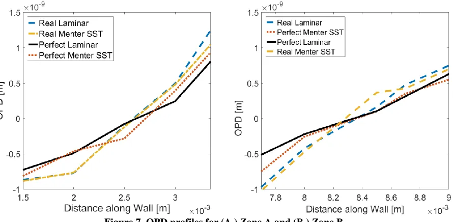
For completeness, the Menter SST model is also run on this case. Because this simplified flow is created to enhance non-equilibrium effects, turbulence does not play a large role in this flow. The turbulent kinetic energy (TKE) is very low for both simulations; the values are less than 7.5 kg∙m2/s2 for the perfect gas simulation and less than 5 kg∙m2/s2 for the real gas simulation. Since turbulent kinetic energy (TKE) is the sum of the turbulent fluctuations in velocity squared, this value can be used as a qualitative measure of how turbulent the flow is. The TKE is higher for the perfect gas simulation. This is consistent with physics, which dictate turbulence is damped by endothermic reactions. The optical calculations are also performed on the Menter SST data; see Fig. 7.
Figure 7. OPD profiles for (A.) Zone A and (B.) Zone B
In Zone A, the real gas Menter SST OPDs are very similar to the laminar results. When plotted, they are nearly indistinguishable from the laminar OPDs for most of the zone. This is unsurprising since there is little turbulence near the stagnation point. In Zone B, all OPDs are also similar. The real gas results have the largest variance in OPD. The perfect gas Menter SST OPDs are mostly larger (in absolute value) than the perfect gas laminar OPDs in Zone B.
B. Effects of Turbulence Modeling
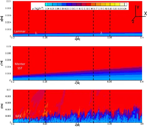
The flow for the turbulence study is typical of a high speed, relatively high Reynolds number, flat plate case. It consists of a weak oblique shock at the leading edge of the plate and a thin boundary layer confined to the area near the wall. Contours of density for all three simulations are shown in Fig. 8. Also show on Fig. 8 is the coordinate axes that will be used in this portion of the study. The figure displays density contours for the laminar simulation, the Menter SST simulation, and the ILES simulation in that order. One should note that the figures do not show the entire flat plate. The only portion of the plate shown is the region where the boundary layer reached turbulent equilibrium. The ILES simulation was run until mean flow statistics converged. Then the average density profiles are compared to that of a fully turbulent boundary layer RANS case as shown in detail in the following section. (the RANS case is fully turbulent and no transition calculations are included). The ILES data taken at z=0.0129 m and at time = 0.25 ms is used for this analysis.
Figure 8. Flat plate density contours (ILES t= 0.25 ms)
Comparing the three sets of results, it can be seen that the boundary layer is thinnest for the laminar case and that the boundary layer produced by the RANS solution is much closer in thickness to the thickest boundary layer, which is produced by the ILES simulation; see Fig. 9 for further illustration.
1.
2.
Laminar
Menter
SST
ILES
Figure 9. Density curves at (A.) x= 0.23 m and (B.) x= 0.33 m
Note that the Menter SST and time averaged ILES curves are in good agreement within the boundary layer. Some disagreements in the data appears as the oblique shock is approached.
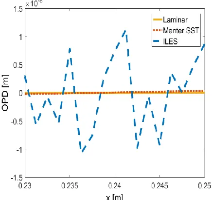
Zones ranging from x = 0.23 m to x = 0.25 m and from x= 0.33 m to x = 0.35 m (labeled 1 and 2 in Fig.8) are extracted to be analyzed for optical properties; specifically, the OPD is calculated for these zones, assuming the beam propagates outward normal to the wall surface. These zones were chosen because they are near the beginning and end of the turbulent zone in the ILES study. The density variation between successive x locations in each zone is very important for optical distortion calculations. Figure 10 shows the density profiles at x=0.23 m, x=0.235 m, and x=0.24 m. Note the significant variation in shape between the various locations for the ILES simulation.
Menter
SST
B. Menter SST
A.
Laminar
A.
B.
Figure 10. Flat plate density profiles for (A.) laminar simulation, (B.) RANS, and (C.) ILES (t=0.25 ms) for Zone 1
The various laminar and Menter SST profiles fall almost on top of each other. The effects of this similarity in profile will be shown later in the small optical path differences for these two simulations. The ILES simulation produces varying density profiles. Three density profiles normal to the wall at x=0.33m, x=0.335m, and x=0.34m are extracted and are plotted; see Fig. 11.
C. ILES
B. Menter SST
A.
Laminar
Figure 11. Flat plate density profiles for (a.) laminar simulation, (b.) RANS, and (c.) ILES (t=0.25 ms) for Zone 2
The data sets from Fig. 11 show the same trends as Fig.10. The laminar and Meter SST profiles do not show many differences at the different x locations. The ILES profiles show fluctuations in density near the wall. Again, the ILES data taken at z=0.0129 m and at time = 0.25 ms is used for this analysis.
The results for the optical calculations for the range of data from x = 0.23 m to x = 0.25 m are shown in Fig. 12. Since it is the variations in flow that distort optical calculations, it is unsurprising thatthe ILES shows the largest OPDs. This can be attributed to the fact that the ILES simulation is the only one that captures fluctuating quantities. While the Menter SST simulation produces a similar boundary layer thicknesses and bulk flow quantities, it is unable to provide fluctuating values, and because of this the OPD profile of this region is not significantly dissimilar to the OPD profile of the laminar solution; both produce tilted linear OPDs that are up to two orders of magnitude lower than the non-linear OPDs predicted from the ILES simulation.
C. ILES
The OPD profiles for Zone 2 are shown in Fig.13. The results are similar to Zone 1. The Menter SST and laminar results basically collapse onto one another; also, with this zone the ILES results can be up to two orders of magnitude larger.
Figure 13. Profiles of OPD for Zone 2 of the flat-plate flow
The data sets for both subzones are taken in such a manner to ensure that all relevant flow features are captured; that is, each data set is taken from the wall extending into the freestream. Because of the large difference between ILES and Menter SST optical solutions, it is unlikely that a Menter SST solution will provide data to produce adequate optical assessments even in thinner boundary layers.
All of the turbulent data shown in Figs. 8-13 are taken at a plane where z=0.0129 m and at time t = 0.25 ms. Data sets are collected at various z-planes and the conclusions that can be drawn from the various z planes are the same. Figure 14 shows OPD maps calculated at various z locations. Because of the similarities between the z planes, all data from other streamwise planes are not shown; no additional conclusion could be drawn from their inclusion. Data is also taken at different time steps. Figure 14 also shows the optical distortions at different times.
Figure 14. Profiles of OPD obtained from the ILES flow simulation: (a) in 3 different streamwise planes (t=0.25 ms); (b) at 3 different time steps (z=0.0129 m)
Figure 14 shows that while the locations of the peaks and troughs in OPD may shift, the magnitude of the fluctuations are similar at all times and streamwise plane locations.
IV. Conclusions and Future Work
For vehicles traveling at hypersonic speeds it is very important to consider flow phenomena that differ from those involved at lower Mach numbers. For example, thermochemical non-equilibrium effects become important as Mach number increases above 5. Until now, it has been unclear whether analysis of the performance of optical sensors in the hypersonic regime would need to be conducted differently than that at lower speeds. This study set out to examine various methods of analyzing hypersonic flow and to determine any effect that the flow field solutions produced by these methods could have on assessment of optical properties.
The study was divided into two portions. The first portion was designed to determine the need for thermochemical non-equilibrium modeling, and the second portion was designed to discern the needed fidelity to model or partially resolve turbulence for optical calculations. A hemisphere flare case was created to determine if equilibrium effects are important to optical calculations. From this study, it was determined that including non-equilibrium effects in the flow field and optical calculations created more variance in the optical path differences. These differences were, however, limited to about a factor of 2. The flat plate simulation was conducted to determine the effects of varying levels of turbulence resolution. This study showed that both laminar and Menter SST simulations produced relatively small, linear OPD profiles. The ILES solution, on the other hand, produced larger and non-linear OPD profiles. These results are unsurprising since ILES is the only method that produces turbulent fluctuating quantities. From the turbulence study, it was deduced that running the more expensive ILES is necessary to capture an accurate description of optical distortion of the flowfield; the simpler Menter SST calculation did not produce OPDs close to those generated by ILES.
These studies did not include both turbulence and thermochemical non-equilibrium in the same simulation. In the future this needs to be completed in order to determine the effects that these phenomena may have on each other and consequently on optical calculations. A few preliminary studies have been conducted on the interaction between turbulence and chemical reactions, and they have shown that turbulence may have a significant effect on detailed chemical composition. These compositions are very important for assessment of optical sensors, as each chemical
A small number of studies that involve only thermal non-equilibrium in turbulent flow have produced different results depending on the physics of the simulation. The physics are often represented as the ratio of the time scales of the turbulence and vibrational relaxation, termed the Damkohler number.16 Depending on this ratio, the turbulent fluctuations can either be damped, or they can be amplified. For example, if the vibrational energy lags behind the translational energy, energy will be transferred out of the turbulent kinetic energy into the vibrational energy; thus, the turbulent fluctuations will be damped.16 The interplay between turbulence, chemistry, and vibrational relaxation must be considered in order to accurately assess the flow around a hypersonic vehicle. The next step in this investigation is to conduct a simulation that includes both thermochemical non-equilibrium effects as well as resolved turbulence.
Acknowledgements
The authors would like to acknowledge the high-speed computational group in the Aerospace Systems Directorate at the Air Force Research Laboratory (AFRL) who provided much assistance as well as access to computational resources. This study was completed, in part, on AFRL’s high performance computing system. DOD HPCMP hours used under a Frontier Project. DISTRIBUTION A. Approved for public release: distribution unlimited. Cleared on 02 May 2017. Case Number: 88ABW-2017-2119.
References
1Gladstone, J. H. and Dale, T. P., “Researches on the refraction, dispersion and sensitiveness of liquids,” Phil. Trans. Royal Soc. London 153, 1864, pp.317–343.
2Weng, M., Mani, A., and Stanislav, G., “Physics and Computation of Aero-Optics,” Annu. Rev. Fluid Mech., Vol. 44, 2012, pp.299-321.
3Martin, A., Scalabrin, L.C., and Boyd, I.D., “High Performance Modeling of Atmospheric Re-entry Vehicles,” Journal of Physics: Conference Series, Vol. 341, 2012.
4Menter, F.,“Improved Two-Equation k-omega Turbulence Models for Aerodynamic Flow,” NASA STI/Recon Technical Report, October 1992.
5Spalart, P.R. and Allmaras, S.R.,“A One Equation Turbulence Model for Aerodynamic Flows,” AIAA-92-0439, January 1992.
6Subbareddy, P.K., and Candler, G.V., “DNS of Transition to Turbulence in a Mach 6 Boundary Layer,” AIAA paper 2012-3106, 2012.
7Park, C. Nonequilibrium Hypersonic Aerothermodynamics, John Wiley & Sons, 1990.
8Landau, L., and Teller, E., “Zur Theorie der Schalldispersion,” Physikalische Zeitschrift der Sowjetunion, Vol, 10, 1936, pp. 34-43
9Millikan, R.C., and White, D.R., “Systematics of Vibrational Relaxation,” Journal of Chemical Physics, Vol. 39, 1963, pp. 3209-3213.
10Handbook of Chemistry and Physics, Edited by David R. Lide, CRC Press, 1996, p. 10-304.
11Anderson, J. H. B.,"An Experimental Determination of the Gladstone-Dale Constants For Dissociating Oxygen," Technical note, 1967.
12Alpher, R.A., and White, D.R., “Optical Refractivity of High Temperature Gases. I. Effects Resulting from Dissociation of Diatomic Gases,” Physics of Fluids, Vol.153, 1958.
13Vogiatzis, K., Josyula, E., and Vedula, P., “Role of High Fidelity Nonequilibrium Modeling in Laminar and Turbulent Flows for High Speed ISR Missions,” AIAA paper 2016-4317, 2016.
14Gerorgiadis, N. J., Rizzetta, D. P., Fureby, C., “Large-Eddy Simulation: Current Capabilities, Recommended Practices, and Future Research,” AIAA Journal 2010 48:8, pp.1772-1784
15Martin, M.P., “Exploratory Studies of Turbulence.Chemistry Interactions in Hypersonic Flows,” AIAA Paper 03-4055, 2003.
16Neville, A.G., Nompelis, I., Subbareddy, P. K., and Candler, G.V., “Effects of Thermal Non-equilibrium on Decaying Isotropic Turbulence,” AIAA Paper 2014-3204, 2014.
17Merzkirch, W., Flow Visualization, 2nd edition, Elsevier, 2012.