©2007 Royal Statistical Society 0035–9254/07/56079 56,Part1,pp.79–97
Model-based estimates of the finite population mean
for two-stage cluster samples with unit
non-response
Ying Yuan
University of Texas M. D. Anderson Cancer Center, Houston, USA
and Roderick J. A. Little
University of Michigan, Ann Arbor, USA
[Received August 2005. Final revision August 2006]
Summary.We propose new model-based methods for unit non-response in two-stage survey samples. A commonly used design-based adjustment weights respondents by the inverse of the estimated response rate in each cluster (method WT). This approach is consistent if the response probabilities are constant within clusters but is potentially inefficient when the esti-mated cluster response rates are very variable. Clusters can be collapsed to increase precision, but this may introduce bias.We consider here the model-based approach to survey inference that treats the clusters as random effects. We note that, from a model-based perspective, a missing data mechanism that assumes that the response rate varies across clusters is non-ignorable, and we propose the term cluster-specific non-ignorable (CSNI) non-response to describe this mechanism. We show that the standard random-effects model estimator RE of the population mean is biased under CSNI non-response, and we propose two modifications of RE to cor-rect this bias. One approach includes the observed response rate as a cluster level covariate (method RERR), and the other is based on a probit model for response (method NI1).The RERR approach is simpler than NI1 but approximate, in that uncertainty in estimating the response rates is not taken into account. In addition, a simple method that corrects the bias of RE by reweighting (method RWRE) is also discussed. We show by simulations that estimators from RERR and NI1 can correct the bias of RE under CSNI non-response and have comparable or lower root-mean-squared error than WT in a variety of simulation settings, and RWRE has similar performance to WT. We also consider another non-ignorable response model estimate of the population mean (NI2) that removes the bias of WT, RWRE, RERR and NI1 under an outcome-specific non-ignorable response mechanism where non-response depends directly on the individual level survey outcomes. However, that estimate is not robust to model mis-specification. The various methods are compared on a data set from the Detroit Dental Health Project.
Keywords: Cluster sampling; Non-ignorable non-response; Random-effects model; Unit non-response
1. Introduction
Statistical adjustments for non-response are increasingly important, given declining response rates in many surveys (De Heer, 1999; Groves and Couper, 1998). This paper concerns unit non-response adjustments in the context of two-stage cluster sampling. Consider a population of sizeMconsisting ofNclusters withMielements in theith cluster. LetYijdenote the value
Address for correspondence: Roderick J. A. Little, Department of Biostatistics, University of Michigan, 1420 Washington Heights, Ann Arbor, MI 48109, USA.
of a survey outcomeYfor unitjin clusteri, fori=1, . . . ,N,j=1, . . . ,Mi, and let
T=N
i=1
Mi
j=1Yij
andY¯=T=Mdenote the population total and mean respectively. At the first stage, a sample of
nof theNclusters (primary sampling units (PSUs)) is selected. At the second stage,miof the Miunits (secondary sampling units (SSUs)) are selected in theith sampled cluster, but onlyri of themisampled units respond. We consider estimates of the finite population meanY¯or total
T. To focus on non-response adjustment, we assume that survey sampling is non-informative in the sense that the selection probability of a unit does not depend on its value ofY. A commonly used design-based approach is to discard the non-respondents and to weight the respondents in theith cluster by the design weight multiplied by the inverse of its response rateri=miin the cluster. This weighting approach is simple, and design consistent if response probabilities are constant within clusters. A weakness of this weighting estimate is that it may have large variance if the weightsmi=riare highly variable; it is not even defined ifri=0 for one or more clustersi. In addition, it is well known that the weighting adjustment yields a biased estimate ofY¯if the response probability of thejth subject in theith cluster depends on the survey outcomeyij.
An alternative approach is to apply a random-effects model to the respondent data, such as the model for two-stage samples that was proposed by Scott and Smith (1969). This approach addresses the potential inefficiency of the weighting estimate by borrowing strength across clus-ters. Unfortunately, we show below that this approach requires that the missing data are missing completely at random, and in particular it doesnotin general yield a consistent estimate of the population mean if the non-response rates vary across the clusters. This fact motivates exten-sions of the Scott and Smith (1969) model that allow the outcome mean to depend on the non-response rate in each cluster. A simulation study is described that compares the estimates and inferences from these models with existing approaches.
Rubin (1976) and Little and Rubin (2002) classified non-response mechanisms into three types: missingness completely at random (MCAR), when the probability of the non-response does not depend on the clusters or survey variables; missingness at random (MAR), when the probability of response depends only on the observed values; non-ignorable non-response, when the probability of the non-response depends on the unobserved values. In the context of two-stage samples, three non-response mechanisms that are of particular interest are
(a) MCAR non-response,
(b) cluster-specific non-response, where the probability of response depends on cluster char-acteristics but not on survey outcomes within clusters, and
(c) outcome-specific non-response that depends directly on the value of missing survey out-comes.
It is clear that outcome-specific non-response is non-ignorable. More surprisingly, we point out that cluster-specific non-response is also non-ignorable in the context of the random-effects models that are considered here.
2. Weighting and model-based methods
2.1. Weighting methods
A standard estimate ofY¯for two-stage samples with complete response is the Horvitz–Thomp-son (Horvitz and ThompHorvitz–Thomp-son, 1952) estimator, which weights cases by the inverse of their probability of selection. With non-response, a naïve approach is to apply this estimator to the respondents, yielding
¯ yHT=
n
i=1
ri
j=1π −1
ij yij
n
i=1
ri
j=1π −1
ij , .1/
where πij is the selection probability of unit j in clusteri, which is determined by the sur-vey design. This approach generally requires the missing data mechanism to be MCAR to be consistent. A popular modification for unit non-response multiplies the sampling weight for respondents by a response weight given by the inverse of the estimated response rate within a weighting class, which is often chosen as the cluster for two-stage cluster samples. Respondent
jin clusterithen receives a weight
wij=.πijφˆi/−1 .2/
where ˆφi=ri=miis the observed response rate in clusteri. We assume here that the sampling weight is constant within clusters, i.e.πij=πi for allj; for a discussion of the case where the sampling weight varies within clusters, see Little and Vartivarian (2002). The weighting estimate WT ofY¯is then
¯ yWT=
n
i=1yÅi:
n
i=1π Å
i: .3/
whereyÅi:=.πiφˆi/−1riy¯i,πÅi:=ri.πiφˆi/−1andy¯iis the respondent mean in clusteri. The variance ofy¯WTis approximated by
V.y¯WT/= 1
n
i=1π Å i: 2 V n
i=1 yÅi:
+ ¯y2 WTV
n
i=1 πi:Å
−2y¯WTcov
n
i=1 yÅi:, n
i=1 πÅi:
: .4/
A consistent estimate of V.y¯WT/ is obtained by replacing the variances and covariances in equation (4) with sample estimates.
The methods that are described here apply to any two-stage sampling scheme, but in our simulations we confine attention to the common design that selects PSUs with probabil-ity proportional to PSU size, and SSUs with probabilprobabil-ity inversely proportional to PSU size (the PPS–inverse PPS design), yielding a design with constant inclusion probabilitiesπij=πfor all
iandj(Kish, 1965). The estimate (1) for this design simplifies to the unweighted mean UW,
¯ yUW=
n
i=1riy¯i
n
i=1ri, and the weighting estimate (3) is
¯
yWT=n−1
n
i=1y¯i:
the sample response rates are very variable. In the extreme, WT is undefined when one or more clusters do not have any respondent. Ways around this difficulty are to compute WT by using only clusters with respondents, or to combine clusters with no respondents with other clusters, but both approaches may lead to bias. A second limitation of WT is that it is biased if the response probability of theijth population member depends on the value of yij. In the next section we describe model-based methods for addressing these limitations.
2.2. Random-effects models
An alternative to WT is to discard non-respondents and to base estimates on predictions from a random-effects model fitted to respondents. A natural model for two-stage samples is that first proposed by Scott and Smith (1969) (method RE), namely
[yij|μi,σ2]=N.μi,σ2/,
[μi|μ,τ2]=N.μ,τ2/, .5/
whereN.·/denotes a normal distribution. RE resolves the potential inefficiency of WT, and the lack of definition of WT when there are clusters with no respondents, by borrowing strength across clusters. Let ˆσ2and ˆτ2denote estimates of the fixed parameters, computed for example by restricted maximum likelihood. For the PPS–inverse PPS design that we consider, larger PSUs are overrepresented in the sample, and valid application of this model requires the assumption that the cluster means are unrelated to size (Sverchkov and Pfeffermann, 2004). To focus on the non-response issue, we make that assumption here and comment on the case where this does not hold in the concluding section. For purposes of prediction under model (5), units of the population fall into three groups. The first group consists of the respondent values, sayyobs, which are known and do not require estimation. The second group consists of the units in clus-ters that are not sampled; these are predicted by the estimate ofμ, which is a weighted mean:
¯ yW=
n
i=1κiy¯i
n
i=1κi, κi= τˆ
2
ˆ
τ2+σˆ2=ri: .6/ The third group consists of the non-respondents and non-sampled units in the sampled clusters; these are estimated by
E.μi|yobs/=κiy¯i+.1−κi/y¯W:
Combining these predictions,Y¯is estimated by
¯
yRE=E.Y¯|yobs/
=M1
n
i=1
ri
j=1yij+
n
i=1.Mi−ri/{κiy¯i+.1−κi/y¯W}+
N
i=n+1Miy¯W
:
The estimated variance ofy¯REis given by Scott and Smith (1969).
random effects; we propose the term cluster-specific non-ignorable (CSNI) non-response to describe this mechanism, to distinguish it from other forms of non-ignorable non-response. A consequence of the non-ignorability is that RE leads to biased estimates in this case (Little and Rubin (2002), example 6.24). The bias comes from two sources. First,y¯W is a biased estimate ofμ. To see this, we rewritey¯Was
¯ yW=
n
i=1
ˆ τ2 ˆ
τ2+.σˆ2=mi/.1=φˆi/y¯i
n
i=1
ˆ τ2 ˆ
τ2+.σˆ2=mi/.1=φˆi/:
Since the non-response probability ofyij depends only on the underlying cluster meansμi, respondents in clusteriare a random sample of elements in this cluster. Thus,y¯iis a consistent estimate ofμi, and the correct weight associated withy¯iis
κi= τˆ
2
ˆ
τ2+σˆ2=mi: .7/
However, the weightκihere is distorted by the different cluster response rate ˆφi, soy¯Wis biased. The larger is the variation of ˆφi, the larger the bias. Second, the predictor of non-respondents and non-sampled elements, κiy¯i+.1−κi/y¯W, adjusts the cluster sample mean towards this biased estimate ofμ. The extent of the adjustment is determined by ˆσ2=τˆ2andri. Ifriis very large,κi≈1, and there is very little adjustment. Ifriis small, large ˆσ2=τˆ2causes more adjustment, and hence more bias. These facts motivate a simple approach to correct the bias by modifying κi to reflect the correct weight. Specifically, we changeκi in equation (6) to that in equation (7). This reweighted random-effects model based approach (method RWRE) yields a consistent estimate ofY¯when non-response depends on cluster means, given that each sampled cluster has at least one respondent. However, if some sampled clusters do not have any respondent, RWRE yields biased estimates, since it ignores these clusters.
The bias of RE when data are not missing completely at random motivates extensions of the RE model for CSNI mechanisms. An informal approach is to modify the RE model to allow the cluster mean to depend on the estimated cluster response rate. Assuming for simplicity a linear relationship yields the approximate model
[yij|αi, ˆφi,σ2]=N.αi+βφˆi,σ2/, [αi|α,τ2]=N.α,τ2/,
which is easily fitted by including the estimated response rate in each cluster as a covariate in the RE model. We label estimates for this model RERR, for the random-effects model with response rate as covariate. This approach is approximate in that the sampling error in estimating the response rate is not taken into account. A more rigorous extension of RE is to model the missing data mechanism directly by the following non-ignorable probit model (NI1):
[yij|αi,χi,β,σ2]=N.αi+βχi,σ2/, [zij|yij,αi,χi]=N.χi, 1/,
rij=
1 ifzij>0, 0 ifzij<0, [αi|χi,α,τ2]=N.α,τ2/,
[χi|χ,ω2]=N.χ,ω2/,
⎫ ⎪ ⎪ ⎪ ⎪ ⎪ ⎪ ⎪ ⎪ ⎬ ⎪ ⎪ ⎪ ⎪ ⎪ ⎪ ⎪ ⎪ ⎭
whererijis the response indicator.rij=1 for respondents andrij=0 for non-respondents. The normal latent variablezijdetermines the response status of the subjectjin the clusteri. If the value ofzij is greater than the threshold 0, the subject responds; otherwise, the subject does not respond. The variance ofzijis set to 1 since the scale of this latent variable is arbitrary and not identifiable. Integrating over the latent{zij}is easily seen to yield a probit model for the missing data process. The latent variable interpretation of the probit model has been discussed by Albert and Chib (1993).
These models assume a CSNI mechanism whererijandyijare unrelated within clusters. An outcome-specific non-ignorable (OSNI) response mechanism assumes that missingness ofyij depends directly on the value ofyij. Such a mechanism is modelled by changing NI1 so thatyij has a linear regression onzijrather than its meanχi, i.e.
[yij|αi,zij,β,σ2]=N.αi+βzij,σ2/, [zij|αi,χi]=N.χi, 1/,
rij=
1 ifzij>0, 0 ifzij<0,
[αi|χi,α,τ2]=N.α,τ2/, [χi|χ,ω2]=N.χ,ω2/:
⎫ ⎪ ⎪ ⎪ ⎪ ⎪ ⎪ ⎪ ⎪ ⎬ ⎪ ⎪ ⎪ ⎪ ⎪ ⎪ ⎪ ⎪ ⎭
.9/
We label this model NI2. This model can be viewed as an extension of the Tobit model (Amemiya, 1984), which is commonly used in econometrics, with random effects to account for the correlation of values of survey outcomes of participants in the same cluster. As in many non-ignorable response models, such as Heckman-type selection models (Heckman, 1976), the estimation ofβ here is heavily driven by the normality assumption of the latent variable and linear relationship betweenyij andzij. Since these assumptions are untestable on the basis of the observed data, subject-matter knowledge or external information may be required to justify the assumptions.
Models (8) and (9) are special cases of the more general model
[yij|zij,αi,β,σ2]=N{αi+λβ.zij−χi/+βχi,σ2}, [zij|χi]=N.χi, 1/,
rij=
1 ifzij>0, 0 ifzij<0, [αi|χi,α,τ2]=N.α,τ2/,
[χi|χ,ω2]=N.χ,ω2/,
⎫ ⎪ ⎪ ⎪ ⎪ ⎪ ⎪ ⎪ ⎪ ⎬ ⎪ ⎪ ⎪ ⎪ ⎪ ⎪ ⎪ ⎪ ⎭
.10/
which yields model (8) whenλ=0 and model (9) whenλ=1. It is tempting to try to fit model (10) to the data, but in practice the parameterλis at best weakly identified. This model might form the basis of a sensitivity analysis with a range of fixed values ofλ, and it is used to generate data for the simulation study in Section 3.
2.3. Fitting the random-effects models
maximum likelihood estimate (Gelmanet al., 2004). Estimates for the RE and RERR models are obtained by the Gibbs sampler (Gelfandet al., 1990). The Gibbs sampler for RE is easily modified for RWRE by applying the modified weights. For example, for RE,μiis drawn from
[μi|yij,μ,σ2,τ2]=N
τ2
τ2+σ2=riy¯i+ σ2=r
i
τ2+σ2=riμ, τ2σ2 riτ2+σ2
:
In contrast, for RWRE,μiis drawn from
[μi|yij,μ,σ2,τ2]=N
τ2
τ2+σ2=miy¯i+
σ2=m
i
τ2+σ2=miμ, τ2σ2 miτ2+σ2
:
We use non-informative priors forμin RE, orαandβin RERR, and diffuse inverse gamma priors forσ2andτ2. In particular for RERR
[α,β,σ2,τ2]∝.σ2/−.a1+1/exp.−b
1=σ2/.τ2/−.a2+1/exp.−b2=τ2/,
witha1=b1=a2=b2=0:1, a value that is sufficiently small that the information in the data strongly dominates the information in the prior distribution. The variance estimator based on the RERR model might fail since RERR is an approximate model. We hence consider a boot-strap variance estimator for RERR, which is less reliant on the model and more consistent with design-based perspectives. For the models NI1 and NI2 we assume priors for the fixed parameters of the form
[β,σ2]∝.σ2/−.a1+1/exp.−b 1=σ2/, [α,τ2]∝.τ2/−.a2+1/exp.−b
2=τ2/, [χ,ω2]∝.ω2/−.a3+1/exp.−b
3=ω2/,
witha1=b1=a2=b2=a3=b3=0:1, again so that the information in the data strongly dom-inates the information in the prior distribution. Computation via the Gibbs sampler is again straightforward, provided that the latent values{zij}are included as missing data. Details of fit-ting NI2 are given in Appendix A. We monitored convergence of the Gibbs chains by graphical inspection, and by the methods of Gelman and Rubin (1992) and Johnson (1996).
3. Simulation study
3.1. Description of study
Eight populations ofM=ΣNi=1Mi=398886 values of a variableYwere constructed in 800 clus-ters. Clusters sizes{Mi}were randomly generated from a uniform distribution with a minimum size of 50 and a maximum size of 1000. The populations were then constructed by using model (10). The parameterβdetermines the degree of non-ignorability of the missing data mechanism. Ifβ=0, the missing data mechanism is MCAR, and larger values ofβcorrespond to stronger degrees of non-ignorability. We simulated populations with two values ofβ,β=0 andβ=10. The parameterλdetermines the extent to which the missing data mechanism depends on the cluster meanχiand the value ofyij itself. Ifλ=1, the missingness ofyij depends entirely on yij, and we have OSNI non-response; ifλ=0, the missingness ofyijonly depends onχi, and
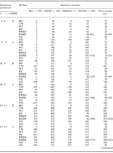
Table 1. Empirical bias, RMSE, change in RMSE relative to BD, average estimate of standard error ESTSE and non-coverage rate of 95% confidence intervals (nominally, target = 25) for seven methods under the (80, 10) design†
Simulation Method Summary outcomes parameters
Bias (×100) RMSE (×100) RRMSE (%) ESTSE (×100) Non-coverage
β λ CORR‡ rate
0 0 H BD −1 58 0 59 23
UW 3 67 14 67 29
WT 1 64 10 64 30
RE −3 64 9 61 32
RWRE 2 64 10 62 29
RERR 2 66 13 69 (65) 24 (30)
NI1 3 66 13 64 28
NI2 2 120 106 120 27
0 0 L BD 1 102 0 105 22
UW −5 127 25 129 23
WT 8 140 37 148 18
RE −6 128 26 121 28
RWRE 8 142 39 145 18
RERR 5 147 44 142 (152) 35 (21)
NI1 9 141 38 151 20
NI2 48 328 221 314 31
10 0 H BD 3 122 0 123 27
UW 415 431 253 119 467
WT 81 145 19 122 49
RE 110 161 32 114 88
RWRE 83 146 20 116 58
RERR −1 124 2 90 (123) 68 (29)
NI1 −5 126 3 127 29
NI2 −180 227 86 123 154
10 0 L BD 7 146 0 154 21
UW 455 483 230 165 396
WT 92 203 38 185 43
RE 326 365 149 164 257
RWRE 94 207 41 182 47
RERR −5 183 25 161 (186) 44 (29)
NI1 15 183 25 187 21
NI2 −851 914 525 332 364
10 0.5 H BD −3 123 0 128 23
UW 680 688 458 108 500
WT 411 423 243 104 491
RE 454 464 277 99 500
RWRE 413 425 245 100 493
RERR 343 358 190 86 (104) 479 (455)
NI1 339 355 188 106 444
NI2 −23 138 12 125 40
10 0.5 L BD 2 159 0 155 26
UW 688 706 344 155 496
WT 427 457 188 171 352
RE 613 632 298 151 489
RWRE 431 462 191 169 359
RERR 340 378 138 160 (173) 280 (251)
NI1 353 391 146 176 268
NI2 −383 512 222 333 98
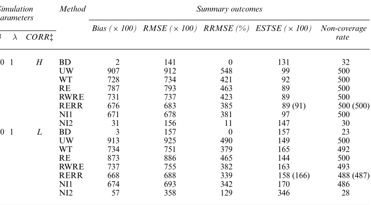
Table 1 (continued)
Simulation Method Summary outcomes parameters
Bias (×100) RMSE (×100) RRMSE (%) ESTSE (×100) Non-coverage
β λ CORR‡ rate
10 1 H BD 2 141 0 131 32
UW 907 912 548 99 500
WT 728 734 421 92 500
RE 787 793 463 89 500
RWRE 731 737 423 89 500
RERR 676 683 385 89 (91) 500 (500)
NI1 671 678 381 97 500
NI2 31 156 11 147 30
10 1 L BD 3 157 0 157 23
UW 913 925 490 149 500
WT 734 751 379 165 492
RE 873 886 465 144 500
RWRE 737 755 382 163 493
RERR 668 688 339 158 (166) 488 (487)
NI1 674 693 342 170 486
NI2 57 358 129 346 28
†Values in parentheses are the corresponding quantities from the bootstrap. ‡H, high;L, low.
the scale of latent variablezij is unidentifiable and arbitrarily set as 1, to obtain differential response rates across clusters, we setχ=1:4 andω2=1. Note that a large value ofω2leads to many clusters that are either all respondents or no respondents, which may not be of interest in practice. The parameterτ2is the variance of the random interceptα
i. We simply set it arbitrarily
at 4 since what is of importance is to control the within-cluster correlation as above. The other parameters in model (10) were chosen so that the superpopulation mean is 40 and the overall response rate is 60%.
Two sampling designs were applied to these populations. In the first, which is denoted the (80, 10) design, a first-stage sample of n=80 PSUs (or clusters) was chosen by probability proportional to size sampling, and a second-stage sample ofm=10 SSUs (or elements) was selected from each sampled PSU, yielding a total sample size of 800. In the second design, which is denoted (20, 40),n=20 PSUs andm=40 SSUs were selected in a similar manner. Each sampling scheme was repeated 500 times for each population and the estimate of the finite popu-lation mean from each method (UW, WT, RE, RWRE, RERR, NI1 and NI2) was com-puted. The unweighted mean before deletion of the missing values (method BD) was also computed as a bench-mark, although of course this method would not be available in practice.
3.2. Results
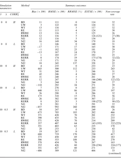
Table 2. Empirical bias, RMSE, change in RMSE relative to BD, average estimate of standard error ESTSE and non-coverage rate of 95% confidence intervals (nominally, target = 25) for seven methods under the (20, 40) design†
Simulation Method Summary outcomes
parameters
Bias (×100) RMSE (×100) RRMSE (%) ESTSE (×100) Non-coverage
β λ CORR‡ rate
0 0 H BD 11 111 0 114 32
UW 3 122 10 124 31
WT 13 116 5 117 32
RE 11 115 4 124 30
RWRE 13 116 5 125 26
RERR 12 116 5 126 (121) 27 (30)
NI1 12 116 5 134 20
NI2 16 149 34 179 18
0 0 L BD 1 146 0 140 31
UW −17 171 17 165 30
WT −1 182 25 181 29
RE −13 167 14 170 27
RWRE 1 185 27 192 25
RERR 0 174 19 175 (174) 32 (32)
NI1 −5 171 18 176 29
NI2 18 345 137 358 22
10 0 H BD 4 235 0 233 23
UW 443 500 112 233 243
WT 31 248 5 246 31
RE 42 246 4 260 27
RWRE 31 248 5 261 28
RERR 12 247 5 146 (240) 122 (32)
NI1 3 244 3 244 27
NI2 −110 292 24 271 39
10 0 L BD 7 276 0 263 21
UW 440 513 86 259 197
WT 26 298 8 286 32
RE 175 318 15 278 56
RWRE 26 302 10 307 22
RERR 8 283 3 198 (272) 98 (32)
NI1 9 281 2 291 22
NI2 −857 992 260 490 186
10 0.5 H BD 10 247 0 249 26
UW 675 705 185 202 466
WT 371 420 70 201 232
RE 390 435 76 211 233
RWRE 371 420 70 214 209
RERR 357 407 64 143 (195) 332 (223)
NI1 351 403 63 225 170
NI2 28 253 2 234 42
10 0.5 L BD 19 267 0 263 22
UW 680 719 170 230 417
WT 375 450 69 250 183
RE 506 553 108 241 270
RWRE 378 454 70 267 163
RERR 352 426 60 196 (236) 224 (177)
NI1 351 427 60 271 133
NI2 −406 589 121 466 33
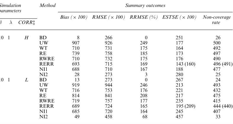
Table 2 (continued)
Simulation Method Summary outcomes
parameters
Bias (×100) RMSE (×100) RRMSE (%) ESTSE (×100) Non-coverage
β λ CORR‡ rate
10 1 H BD 8 266 0 251 26
UW 907 926 249 177 500
WT 710 731 175 164 492
RE 739 758 185 173 497
RWRE 710 732 175 176 490
RERR 693 715 169 143 (160) 496 (491)
NI1 688 710 167 188 477
NI2 28 273 3 280 25
10 1 L BD 13 273 0 267 24
UW 919 944 246 213 493
WT 716 753 176 221 432
RE 814 841 208 217 475
RWRE 719 757 177 235 415
RERR 689 724 165 195 (209) 444 (440)
NI1 685 720 164 245 407
NI2 49 458 68 457 33
†Values in parentheses are the corresponding quantities from the bootstrap. ‡H, high;L, low.
RRMSE=100{RMSE(estimator)−RMSE(BD)}=RMSE(BD),
the average estimated standard error ESTSE, which is the average of the estimated standard errors over the 500 samples, and 95% confidence interval non-coverage rate (nominally, we expect 25). Table 2 shows the results for the (20, 40) design.
3.2.1. Missingness completely at random (β=0)
All methods are consistent when the non-response mechanism is MCAR. RE has the smallest RMSE, reflecting gains in efficiency from shrinkage. UW, WT, RWRE, RERR and NI1 are comparable in terms of RMSE and coverage. NI2 has satisfactory coverage but is less efficient than the other methods.
3.2.2. Cluster-specific non-ignorable non-response (β=10,λ=0)
The missingness ofyij depends only on the cluster meanχi in this CSNI non-response case. UW has large bias and RMSE because of the lack of a non-response adjustment. WT has a slight bias and undercoverage for the (80, 10) design, which comes from dropping clusters with no respondents. RE has a substantial bias and poor coverage in this case since the missing data mechanism is not MCAR as discussed in Section 2.2. The bias of RE is larger when the within-cluster correlation is low and the number of SSUs is small. RWRE corrects or nearly corrects the bias of RE and has very similar performance to WT. It also has a slight bias and undercoverage for the (80, 10) design, since RWRE drops clusters with no respon-dents.
the model-based estimate of variance of RERR leads to confidence intervals that undercover the population mean. The bootstrap variance estimate leads to coverages that are closer to the nominal rate, suggesting that the bootstrap variance estimate is robust to the model misspecifi-cation that is caused by the approximation. NI2 has large bias and RMSE, especially when the within-cluster correlation is low, suggesting the sensitivity of this method to the misspecification of the missingness mechanism.
3.2.3. Outcome-specific non-ignorable non-response (β=10,λ=1)
In this OSNI non-response situation, non-response is related to individual outcomes within clusters, and NI2 is the only method that correctly specifies the OSNI mechanism. As a result, NI2 is the best method in term of RMSE and coverage, and the other methods all perform poorly, although RERR and NI1 outperform WT, RE and RWRE in terms of bias and RMSE.
3.2.4. Mixed cluster-specific and outcome-specific non-ignorable non-response (β=10,λ=0.5)
This mixed CSNI and OSNI non-ignorable missingness mechanism is somewhere between the above two extreme cases withλ=0 andλ=1. None of the methods are satisfactory, although NI2 does relatively well in the case of high within-cluster correlation. Thus there is no single method that dominates the others consistently over all simulation conditions.
4. Application
The Detroit Research Center on Oral Health Disparities at the University of Michigan School of Dentistry (also known as the Detroit Dental Health Project) is a multidisciplinary project that seeks to understand how the broader social context in which families live affects their oral health and well-being, and to design interventions that can have a positive effect within these contexts. The principal theme of the project is to investigate why some African-American children and their main care givers have better oral health than others who live in the same community.
A two-stage equal probability sample was drawn from the 392 000 census tracts within Wayne County, Michigan, with the highest proportion of African-American households with income less than twice the poverty threshold. Blocks within each targeted tract were listed by tract and block number and a probability proportional to size selection method was implemented to select blocks for listing. A total of 118 blocks were selected across the 39 tracts. At the second stage, housing units within segments were selected by simple random sampling with the selec-tion probabilities such that each housing unit has equal probability of selecselec-tion, resulting in 12 655 housing units selected for screening. The two main eligibility criteria were
(a) the household had at least one African-American child under the age of 6 years living in the household and
(b) the family’s income is below 250% of the poverty level.
3.0 3.2 3.4 3.6 3.8
20 40 60
8
0 100
Cluster Sample Mean of log(BMI)
E
s
tim
a
ted Cl
us
ter Re
s
pon
s
e R
a
te (
%
[image:13.485.103.392.56.319.2])
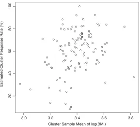
Fig. 1. Sample cluster mean of log(BMI) against estimated cluster response rate
rate was about 40%. Item non-response arose when households failed to answer some questions in the questionnaire but, for most questions, the item non-response rate was less than 5%.
Table 3. Estimates of the finite population mean of log(BMI) by various methods for the oral health disparities data†
Estimate Results for the following methods:
UW WT RE RWRE RERR NI1 NI2
ˆ
¯
Y 3.404 3.392 3.403 3.394 3.390 3.394 3.024
ESTSE( ˆY¯) 0.0079 0.0103 0.0076 0.0078 0.0125 (0.0128) 0.0100 0.0265
† ˆY¯is the estimate of the population mean of log(BMI), and ESTSE( ˆY¯) is the estimate of the associated standard error. The value in parentheses is the corresponding quantity from the bootstrap.
Although we cannot distinguish CSNI and OSNI statistically, we may understand the missing data mechanism from behavioural origins of non-response. In this particular study, the survey design requires fieldworkers to try to ask for the reason of refusal when eligible households refuse to participate in the study. Although only part of these households give the reason for refusal, we note that one major reason that eligible households refused to participate in the study is that they had jobs providing dental insurance. Since higher education is associated with lower BMI, and households with higher education are more likely to have a job with dental insurance, we might expect a positive relationship between BMI and response rate. Because education is an individual characteristic, we speculate that non-response is more likely to be related to an outcome variable, and non-response is OSNI non-response. If we have to choose a single model to report, we may favour the NI2 model.
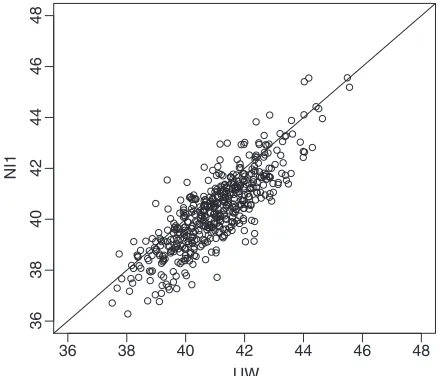
Since this example did not give much indication of bias, we also ran a simulation under the CSNI mechanism that yielded a correlation between the outcome and the response rate which was comparable with that in this data set, and we compared the NI1 and UW estimates over 500 repeated samples. The UW method exhibited bias and undercoverage overall, but the estimates for the two methods were similar for a substantial fraction of the data sets as shown by Fig. 2, illustrating that properties cannot be inferred from the results of a single data set.
36 38 40 42 44 46 48
3
6
38
40
42
44
46
4
8
UW
NI1
[image:14.485.131.353.422.610.2]5. Conclusion
This paper proposes several model-based estimates of the finite population mean for two-stage samples with unit non-response and compares them with existing methods by a simulation study. When the non-response mechanism is MCAR, all methods are consistent, but RE has the smallest RMSE owing to gains in efficiency from shrinkage. When non-response depends on cluster means, UW and RE are subject to bias. WT is consistent but can be inefficient if cluster response rates are variable. RWRE is a simple method to correct the bias of RE when non-response depends on clusters, but, like WT, it may fail in the presence of clusters with-out respondents. RWRE and WT have similar performances since the reweighting procedure in RWRE is to adjust weights of responses to reflect the correct weights, following the same reasoning as for WT. This similarity is especially pronounced in equal selection probability designs as in our simulation studies. In this case, the estimate of population mean in equation (6) is the same as WT since the adjustedκiin equation (7) is constant across clusters. RERR is an approximate method to correct the bias of RE when non-response depends on clusters. It overcomes the drawback of RWRE and also gives a solution to the potentially low ineffi-ciency of WT by borrowing strength across clusters in this case. In our simulations, RERR has a smaller RMSE than RE, RWRE and WT. A more rigorous extension of RE when non-response depends on clusters is NI1, which yields estimates that are similar to those from RERR. If the non-response depends on survey outcome, UW, WT, RE, RWRE, RERR and NI1 all have large bias and large RMSE. NI2 addresses this problem and yields consistent estimates. Although non-ignorable response models like NI1 and NI2 are attractive, we should be cautious in applying them because they are sensitive to the misspecification of the missing data mech-anism, the normality assumption of the latent variable and the functional form between the outcome variable and the latent variable. Since these assumptions are untestable on the basis of the observed data, subject-matter knowledge or external information may be required to justify the assumptions.
A natural and important question given these findings is whether we can determine whether the non-response mechanism is MCAR, CSNI or OSNI, and which model should be used. A plot of cluster sample response rates against cluster sample means is useful for helping to understand the relationship between cluster response rates and cluster means. More formally, we can fit a linear regression model or nonparametric smooths and can test the relationship between cluster response rates and cluster means. If there is no significant relationship between cluster response rates and cluster means, RE may be justified. If the relationship is linear, then RERR may be used to reflect this relationship. If the relationship is non-linear, we may consider modelling it by using polynomial or spline techniques. Unfortunately, we cannot distinguish non-response depending on cluster means from non-response depending on outcomes from the plot. However, if auxiliary variables for non-respondents and respondents are available, e.g. from census data, then we could compare the distribution of auxiliary variables of non-respondents with that of respondents within a cluster. If there is no systematic difference, we might assume that non-response is more likely to depend on cluster means and apply WT, RWRE, RERR or NI1; otherwise, we may consider NI2. Since we do not have enough information to distin-guish between alternative non-ignorable missingness mechanisms, it may be more appropriate to apply more than one method and to compare results.
non-response can arise if the cause of the non-response is the value of the survey variable itself or when causes of non-response are also causes of survey variables. The former case is most likely in self-administered questionnaire surveys. With this survey design, the householders have the opportunity to review the entire questionnaire before making the decision to participate. If the underlying cause of refusal to participate is the psychological threat that is posed by the topic in the survey, then the resulting non-response is most likely to be OSNI since the sample subjects’ attributes on the survey variable are determining their probability of partici-pating. In contrast, non-response in many interview-administrated surveys may be less directly related to the survey variables because the respondent has only a general idea about the topic of the survey. Nevertheless, as Groves and Couper (1998) noted, survey-specific characteristics may cause interview-administrated surveys to be specifically subject to OSNI non-response. For example, time use surveys measuring how people spend their time would be highly susceptible to non-contact non-response. Individuals who are away from home most of the time are more likely to be non-respondents through non-contact and are systematically different from others in ‘away-from-home’ activities, i.e. non-response directly depends on survey variables themselves. It is probably more common that the survey variables that are measured do not cause non-response, but, instead, non-reponse and survey variables share a common possible unobserved cause. In these circumstances, CSNI non-response arises when the common cause is a cluster level characteristic (or covariate). If the common cause is an individual level characteristic (or covariate), OSNI non-response results. An example of this might be a two-stage cluster sam-ple with schools as PSUs and students as SSUs. If non-response of students is deemed to be related to school level variables (e.g. school location, financial situation or goodness of admin-istration) that are also associated with survey variables of interest, then the non-response is CSNI. However, if the non-response of students depends on individual characteristics such as a student’s personality or academic performance, which also affect the survey variables, then the non-response is OSNI. Of course, if the common cause variable is known for both respon-dents and non-responrespon-dents, by conditioning on it, the non-ignorability of non-response can be largely removed. When designing and implementing surveys, it is important to anticipate systematic relationships between attributes of the survey request, the participant’s decision to participate and the survey variable of interest, both for reduction of non-response and post-sur-vey non-response adjustment (Groves and Couper, 1998). Understanding these relationships greatly helps us to identify CSNI and OSNI non-response and to choose appropriate models like NI1 or NI2 to achieve valid inference.
This paper focuses on two-stage cluster samples, but our models can be readily extended to accommodate multistage cluster samples. To reflect the design feature of multistage cluster sam-pling, we can use multilevel hierarchical models where different level within-cluster correlations are modelled by different level random effects. In this case, CNSI and OSNI non-response arise when non-response depends on clusters’ characteristics or survey outcomes respectively. It is straightforward to adjust for OSNI non-response. The same latent variable approach as NI2 can be used to model the OSNI missing data mechanism. For CSNI non-response, the situation is a little complex. In the context of multilevel hierarchical models, CSNI non-response can associate with underlying cluster characteristics at different levels. In principle, we could extend the NI1 model to allow the mean of outcome variable to depend on random effects of all levels. However, since substantial within-cluster correlation may occur in only certain levels and also for the convenience of estimation, it may be adequate just to model the relationship between outcome variables and random effects of these levels.
design and the weights are solely attributable to non-response. However, from equation (2), it is clear that if there are sampling weights, as in many survey designs, WT will be more variable; then the RE and RERR methods have greater potential for gains in efficiency. For simplicity, we have considered random-effects models that condition on cluster response rates alone, since this relationship is particularly important from the point of view of a consistent estimate of the population mean (Little and An, 2004). Other cluster level characteristics could be added to our models as covariates if available. In particular, we have assumed here that the size variable determining the first-stage selection probability is unrelated to the outcome. This assumption can be relaxed by including the size variable as a covariate in the random-effects model.
Acknowledgements
This paper was supported by grant DMS 0106914 from the National Science Foundation. The authors thank Amid I. Ismail at the School of Dentistry at the University of Michigan for pro-viding the Detroit dental health data. The authors also thank three referees and the Associate Editor for their insightful and detailed comments that improved this paper.
Appendix A: Gibbs sampler
Let yobs andymis denote values of the survey outcome Y for respondents and non-respondents, and
z={zij},i=1, . . . ,n,j=1, . . . ,mi, denote values of the latent variable. Consider thekth iteration of the Gibbs sampler. For non-ignorable response model NI2, the first step of the iteration is ‘data
augmenta-tion’ (Tanner and Wong, 1987), in which the missingyijand latent variablezijare generated from their full
conditional distributions. Whenrij=1, i.e.yijis observed,zijis drawn from the following left-truncated
normal distribution TN:
[zij|yobs,rij=1,αi,β,χi,σ2]=TN[zij>0]
χi+β2+βσ2.yij−αi−βχi/, σ2 β2+σ2
:
Whenrij=0,.yij,zij/are drawn from the conditional distributions
[zij|yobs,rij=0,αi,β,χi,σ2]=TN[zij<0].χi, 1/,
[yij|yobs,z,rij=0,αi,β,σ2]=N.αi+βzij,σ2/:
Now, with augmented complete data.yobs,ymis,z/, parameters are drawn alternately.
α={αi},i=1, . . . ,n, is drawn from the conditional distribution
[αi|yobs,ymis,z,α,β,σ2,τ2]=N
miτ2.y¯
i−βzi/¯ +σ2α miτ2+σ2 ,
σ2τ2 miτ2+σ2
where
¯ yi=
1 mi
mi
j=1
yij
and
¯ zi=
1 mi
mi
j=1
zij:
χ={χi},i=1, . . . ,n, is drawn from the conditional distribution
[χi|yobs,ymis,z,χ,ω2]=N
miω2¯zi+χ miω2+1
, ω
2
miω2+1
:
[σ2|yobs,ymis,z,α]=IG
a1+
1 2
n
i=1 mi−1
,b1+
1 2 n i=1
mi
j=1
.yij−αi−βˆzij/2
,
[β|yobs,ymis,z,α,σ2]=N
⎧ ⎨ ⎩βˆ,
n i=1
mi
j=1 z2 ij −1 σ2 ⎫ ⎬ ⎭ where ˆ β=n
i=1 mi
j=1
zij.yij−αi/
n i=1
mi
j=1 z2
ij,
and IG(·) denotes an inverse gamma distribution.
.α,τ2/are drawn from the conditional distributions
[τ2|y
obs,ymis,z,α]=IG
a2+
1
2.n−1/,b2+
1 2
n i=1
.αi− ¯α/2
,
[α|yobs,ymis,z,α,τ2]=N
¯ α,τ
2
n
where
¯ α=1
n n i=1
αi:
.χ,ω2/are drawn from the conditional distributions
[ω2|yobs,ymis,z,χ]=IG
a3+
1
2.n−1/,b3+
1 2
n i=1
.χi− ¯χ/2
,
[χ|yobs,ymis,z,χ,ω2]=N
¯ χ,ω
2
n
where
¯ χ=1nn
i=1 χi:
References
Albert, J. and Chib, S. (1993) Bayesian analysis of binary and polychotomous response data.J. Am. Statist. Ass.,
88, 669–679.
Amemiya, T. (1984) Tobit models: a survey.J. Econometr.,24, 3–61.
De Heer, W. (1999) International response trends: results of an international survey.J. Off. Statist.,15, 129–142. Gelfand, A. E., Hills, S. E., Racine-Poon, A. and Smith, A. F. M. (1990) Illustration of Bayesian inference in
normal data models using Gibbs sampling.J. Am. Statist. Ass.,85, 972–985.
Gelman, A., Carlin, J. B., Stern, H. S. and Rubin, D. B. (2004)Bayesian Data Analysis, 2nd edn. New York:
Chapman and Hall.
Gelman, A. and Rubin, D. B. (1992) Inference from iterative simulation using multiple sequences.Statist. Sci.,7, 457–511.
Groves, R. M. and Couper, M. P. (1998)Nonresponse in Household Interview Surveys. New York: Wiley.
Heckman, J. I. (1976) The common structure of statistical models of truncation, sample selection and limited dependent variables and a simple estimator for such models.Ann. Econ. Socl Measmnt,5, 475–492.
Horvitz, D. G. and Thompson, D. J. (1952) A generalization of sampling without replacement from a finite population.J. Am. Statist. Ass.,47, 663–685.
Johnson, V. E. (1996) Studying convergence of Markov Chain Monte Carlo algorithms using coupled sampled paths.J. Am. Statist. Ass.,91, 154–166.
Kish, L. (1965)Survey Sampling. New York: Wiley.
Krosnick, J. A. (1991) Response strategies for coping with the cognitive demands of attitude measures in surveys.
Appl. Cogn. Psychol.,5, 213–236.
Little, R. J. A. (2004) To model or not to model?: competing modes of inference for finite population sampling.
J. Am. Statist. Ass.,99, 546–556.
Little, R. J. A. and An, H. (2004) Robust likelihood-based analysis of multivariate data with missing values.
Statist. Sin.,14, 949–968.
Little, R. J. A. and Rubin, D. B. (2002)Statistical Analysis with Missing Data, 2nd edn. New York: Wiley. Little, R. J. A. and Vartivarian, S. (2002) On weighting the rates in nonresponse weights.Statist. Med.,22,
1589–1599.
Rubin, D. B. (1976) Inference and missing data (with discussion).Biometrika,63, 581–592.
Scott, A. and Smith, T. M. F. (1969) Estimation in multi-stage surveys.J. Am. Statist. Ass.,64, 830–840. Sverchkov, M. and Pfeffermann, D. (2004) Prediction of finite population totals based on the sample distribution.
Surv. Methodol.,30, 79–92.
Tanner, M. A. and Wong, W. H. (1987) The calculation of posterior distributions by data augmentation.J. Am.