A superlinearly convergent SSDP algorithm for nonlinear semidefinite programming

R E S E A R C H

Open Access

A superlinearly convergent SSDP algorithm

for nonlinear semidefinite programming

Jian Ling Li

_{and Hui Zhang}

*_{Correspondence:}

jianlingli@126.com

1_{College of Mathematics and} Information Science, Guangxi University, Nanning, China

Abstract

In this paper, we present a sequential semidefinite programming (SSDP) algorithm for nonlinear semidefinite programming. At each iteration, a linear semidefinite

programming subproblem and a modified quadratic semidefinite programming subproblem are solved to generate a master search direction. In order to avoid Maratos effect, a second-order correction direction is determined by solving a new quadratic programming. And then a penalty function is used as a merit function for arc search. The superlinear convergence is shown under the strict complementarity and the strong second-order sufficient conditions with the sigma term. Finally, some preliminary numerical results are reported.

Keywords: Nonlinear semidefinite programming; Penalty function; Sequential semidefinite programming; Global convergence; Superlinear convergence

1 Introduction

Consider the following nonlinear semidefinite programming (NLSDP) with a negative semidefinite matrix constraint:

min f(x)

s.t. A(x)0,

(1.1)

wheref :Rn→R,A:Rn→Sm,Smis the set ofm-order symmetric matrix andSm₊ (Sm_–) is the set ofm-order positive (negative) semidefinite matrix.A(x)0 means thatA(x) is a negative semidefinite matrix.

Nonlinear semidefinite programming has many applications both in theory and in the real world. Many convex optimization problems, such as variational inequality problems, fixed point problems [1–3], can be reformulated as convex NLSDP. Robust control prob-lems, optimal structural design, and truss design problems can be reformulated as NLSDP (see [4–6]). There are a lot of literature for NLSDP on algorithms, for example, the aug-mented Lagrangian method [7–12], primal-dual interior point method [13,14], and se-quential semidefinite programming (SSDP) method [15–21]. Our research focus is on the SSDP method.

SSDP method, which is a generalization of SQP method for classic nonlinear program-ming, is one of effective methods for nonlinear semidefinite programming. For example,

Correa and Ramirez [16] proposed a global SSDP algorithm for NLSDP. Recently, as illus-trated by the extensive numerical experiments in [20,21], SSDP algorithm has performed very well in finding a solution to NLSDP. At each iteration of SSDP method, a special quadratic semidefinite programming subproblem is solved to generate a search direction. However, just as traditional SQP method, most of existing SSDP methods also have some inherent pitfalls, e.g., (1) the first direction finding subproblem (DFP for short), namely a quadratic semidefinite programming (QSDP for short), is not ensured to be consistent. The algorithm in [21] is based on the assumption that the optimal solution of the first DFP exists. The algorithm in [20] directly goes to feasibility restoration phase when the first DFP is inconsistent. As we know, feasibility restoration phase will increase the com-putational cost. (2) The optimal solution to the first DFP is not ensured to be an improving direction, so it is possible that Maratos effect occurs. As a result, the superlinear conver-gence is not guaranteed to obtain.

Since NLSDP contains a negative semidefinite matrix constraint, it is more difficult to deal with these drawbacks comparing with SQP method for classic nonlinear program-ming. In this paper, we borrow the ideas of modified strategy of quadratic programming subproblem for nonlinear programming from [22]. We first construct a linear semidefi-nite programming (LSDP for short), and then by means of the solution of the LSDP we construct a special QSDP to yield the master search direction, which is ensured to be con-sistent. In order to avoid the Maratos effect, a second-order correction direction is intro-duced which is determined by solving a new quadratic programming. A penalty function is used as a merit function for arc search. The proposed algorithm possesses superlin-ear convergence under the strict complementarity and the strong second-order sufficient conditions with the sigma term.

The paper is organized as follows. Some notations and preliminaries are described in the next section. In Sect.3, we present our algorithm in detail and analyze its feasibility. Under some mild conditions, the global convergence and superlinear convergence are shown in Sect.4and Sect.5, respectively. In Sect.6, the preliminary numerical results are reported. Some concluding remarks are given in the last section.

2 Preliminaries

In this section, for the sake of convenience, some definitions, notations, and results for NLSDP are introduced.

The differential operatorDA(x) :Rn→Smis defined by

DA(x)d:=

n

i=1

di ∂A(x)

∂xi

, ∀d∈Rn. (2.1)

The adjoint operatorDA(x)∗ofDA(x) is defined by

DA(x)∗_Z=∂A(x) ∂x1

,Z

, . . . ,

∂A(x)

∂xn

,Z

T

, ∀Z∈Sm, (2.2)

The operatorD2_{A(x) :R}n_×Rn_→Sm_{is defined by}

dTD2A(x)d¯:=

n

i,j=1

did¯j ∂2_A(x)

∂xi∂xj

, ∀d,d¯∈Rn. (2.3)

Definition 2.1 Givenx∈Rn_{, if there exists a matrixΛ∈S}m

+ such that

∇f(x) +DA(x)∗Λ= 0, (2.4a)

A(x)0, (2.4b)

TrΛA(x)= 0, (2.4c)

thenxis called a KKT point of NLSDP (1.1), the matrixΛis called the Lagrangian multi-plier, (2.4a)–(2.4c) is called the KKT conditions of NLSDP (1.1).

Letλ1, . . . ,λnbe the eigenvalues ofA(∈Rn×n), and letλ1(A) be the largest eigenvalue of

A. The following results will be used in the subsequent analysis.

Lemma 2.1([23]) For any A,B∈Sm,the following inequality is true:

Tr(AB)≤

m

i=1

λi(A)λi(B), (2.5)

the equality holds if and only if there exists an invertible matrix P such that P–1_{AP and}

P–1_{BP are diagonal.}

Based on Lemma2.1, the following result is obvious.

Lemma 2.2 For any A∈Sm,B∈Sm₊,the following inequality is true:

Tr(AB)≤λ1(A)Tr(B). (2.6)

Lemma 2.3([24] (Weyl’s inequality)) Suppose A,B∈Sm_,thenλ

1(A+B)≤λ1(A) +λ1(B).

Lemma 2.4 For any A,B∈Sm_,ifλ

1(A+B) <λ1(A),then the following inequality is true:

λ1(A+ηB)≤λ1(A), ∀η∈(0, 1).

Proof Ifλ1(B)≤0, then it follows from Lemma2.3that

λ1(A+ηB)≤λ1(A) +λ1(ηB)≤λ1(A),

that is, the result is true.

Ifλ1(B) > 0, note thatλ1(A+B) <λ1(A) andη∈(0, 1), then it follows from Lemma2.3

that

λ1(A+ηB) =λ1

A+B+ (η– 1)B

≤λ1(A+B) +λ1

≤λ1(A) + (η– 1)λ1(B)

≤λ1(A),

so the result is proved.

Letxk_{be the current iterative point, motivated by the idea in [22], we construct a linear}

SDP subproblem (LSDP) as follows:

LSDPxk _{min z}

s.t. Axk+DAxkdzEm, (2.7)

z≥0, d ≤1,

whereEmis them-order identity matrix.

It is known thatLSDP(xk_{) (2.7) has optimal solutions. Let ((d}k₎T_,z

k)T be an optimal

solution of LSDP(xk_{) (2.7). Now we construct a quadratic semidefinite programming}

(QSDP(xk_,H

k)) by means ofzkas follows:

QSDPxk,Hk

min ∇fxkTd+1 2d

T_H

kd

s.t. Axk+DAxkdzkEm,

(2.8)

whereHk∈Sn is the Hesse matrix or an approximation of the Hesse matrix of the

La-grangian function of NLSDP (1.1) atxk_.

Generally, the optimal solutiondk_toQSDP(xk_,H

k) (2.8) cannot be guaranteed to avoid

the Maratos effect and get superlinear convergence, so it needs a modification. To this end, motivated by the ideas in [20], we introduce a second-order correction direction by solving the following subproblem:

min ∇fxkTdk+d+1 2

dk+dTHk

dk+d

s.t. N¯_kTAxk+dk+DAxkdN¯k= –dk

Em–r,

(2.9)

where ∈ (2, 3), r =rank(A(xk_{) + DA(x}k_)dk_{), N}¯

k = (pk1,pk2, . . . ,pkm–r)∈ Rm×(m–r), and {pk

1,pk2, . . . ,pkm–r}is an orthogonal basis for the null space of the matrixA(xk) +DA(xk)dk.

The following basic assumptions are required.

A 1 The functionsf(x) andA(x) are continuously differentiable.

A 2 There exist two positive constantsaanda¯such that

ad2≤dTHkd≤ ¯ad2, ∀d∈Rn.

Under Assumptions A1–A2, the following lemma follows.

Lemma 2.5 Suppose that AssumptionsA1–A2hold.Then subproblemQSDP(xk,Hk) (2.8)

has a unique solution dk_{,and there exists a matrixΛ}

ofQSDP(xk_,H

k) (2.8),i.e.,

∇fxk+DAxk∗Λk+Hkdk= 0, (2.10a)

Axk+DAxkdkzkEm, (2.10b)

TrΛk

Axk+DAxkdk–zkEm

= 0. (2.10c)

Define a measure of constraint violation for NLSDP (1.1) as follows:

P(x) =λ1

A(x)₊, (2.11)

whereλ1(A(x))+=max{λ1(A(x)), 0}. Obviously,P(x) = 0 if and only ifxis a feasible point

of NLSDP (1.1).

By means ofP(x), we define a penalty function as a merit function for arc search:

θα(x) =f(x) +αP(x) =f(x) +αλ1

A(x)₊, (2.12)

whereα> 0 is a penalty parameter. The functionθα(x) comes from the Han penalty

func-tion for nonlinear programming.

Lemma 2.6 Suppose that AssumptionsA1–A2hold,dkis the optimal solution ofQSDP(xk, Hk) (2.8).Then the directional derivativeθα(xk;dk)satisfies the following inequality:

θ_αxk;dk

≤ ∇fxkTdk–αλ1

Axk₊–λ1(zkEm)+

(2.13)

≤–dkTHkdk+Tr

Λk

Axk–zkEm

–αλ1

Axk₊–λ1(zkEm)+

, (2.14)

where zkis the optimal value ofLSDP(xk) (2.7),Λk is a KKT multiplier ofQSDP(xk,Hk)

(2.8)corresponding to the constraint.

Proof First, it follows from (2.10a) that

fxkTdk= –

n

i=1

dk_iTr

Λk

∂A(xk) ∂xi

–dkTHkdk. (2.15)

Sinceλ1(·)+is convex, we obtain

λ1

Axk+t

n

i=1

dk_i∂A(x

k₎

∂xi

+

≤(1 –t)λ1

Axk₊+tλ1

Axk+

n

i=1

dk_i∂A(x

k₎

∂xi

+

≤(1 –t)λ1

the last inequality above is due to (2.10b). By the definition of directional derivative and the above inequality, we get

λ1(·)+

_A

xk;DAxkdk

= lim

t→0+t

–1

λ1

Axk+t

n

i=1

d_ik∂A(x

k₎

∂xi

+

–λ1

Axk₊

≤ lim

t→0+t

–1_{(1 –t)λ} 1

Axk₊+tλ1(zkEm)+–λ1

Axk₊ = –λ1

Axk₊–λ1(zkEm)+

. (2.16)

Combining with the definition of the directional derivativeθ_α(xk_;dk_{) and (2.16), we have}

θ_αxk;dk=fxkTdk+αλ1(·)+

_A

xk;DAxkdk

≤fxkTdk–αλ1

Axk₊–λ1(zkEm)+

,

that is, inequality (2.13) holds. By (2.15), we obtain

fxkTdk–αλ1

Axk₊–λ1(zkEm)+

≤–

n

i=1

dk_iTr

Λk

∂A(xk) ∂xi

–dkTHkdk–α

λ1

Axk₊–λ1(zkEm)+

. (2.17)

It follows from (2.10c) that

–Tr Λk _n i=1 dk i

∂A(xk) ∂xi

= –TrΛk

DAxk_dk_=TrΛ k

Axk_–z kEm

. (2.18)

Substituting the above equality into (2.17), one has

fxkTdk–αλ1

Axk₊–λ1(zkEm)+

≤–dkTHkdk+Tr

Λk

Axk–zkEm

–αλ1

Axk₊–λ1(zkEm)+

,

that is, inequality (2.14) holds.

3 The algorithm

In this section, we first present our algorithm in detail, and then analyze its feasibility.

Algorithm A

Step 0. Givenx0∈Rn,H0=En(identity matrix),t∈(0, 1),α0> 0,P¯∈(1, 10),σ∈(0, 1),

β∈(0,1₂),η1> 0. Letk:= 0.

Step 1. SolveLSDP(xk_{)(2.7) to get an optimal solution((d}k₎T_,z

k)T. Ifλ1(A(xk)) > 0and

zk=λ1(A(xk)), then stop.

Step 2. (Generate a master direction). SolveQSDP(xk,Hk)(2.8) to get the optimal

Step 3. (Generate a second-order correction direction). Solve subproblem (2.9) and let

dk_{be the solution. If there is no solution of subproblem (2.9) ord}k_>dk_{, then}

setdk_{= 0.}

Step 4. (Updateαk) The update rule ofαkis as follows:

αk+1:=

⎧ ⎨ ⎩

αk, if(xk,αk)≤–(dk)THkdk;

f(xk₎T_dk_+(dk₎T_H

kdk

λ1(A(xk))+–zk +η1, otherwise,

(3.1)

where(xk_,α

k)is defined by

xk,αk

=fxkTdk–αk

λ1

Axk₊–λ1(zkEm)+

, (3.2)

that is,(xk_,α

k)is the right-hand side of inequality (2.13).

Step 5. (Arc search) Lettkbe the first number of the sequence{1,σ,σ2, . . .}satisfying the

following inequalities:

θαk+1

xk+tkdk+t2kdk

≤θαk+1

xk+βtk

xk,αk+1

, ifPxk≤ ¯P; (3.3)

⎧ ⎨ ⎩

θαk+1(x

k_+t

kdk+t_k2dk)≤θαk+1(x

k_{) +βt}

k(xk,αk+1),

P(xk+tkdk)≤P(xk),

ifPxk>P.¯ (3.4)

Step 6. Letxk+1_:=xk_+t

kdk+t2_kdk, updateHkby some method toHk+1such thatHk+1is

positive definite. Setk:=k+ 1, and return to Step 1.

Remark In Algorithm A, by means of new modified strategies of subproblem, the quadratic semidefinite programming subproblem (2.8) yielding master searching direc-tion is guaranteed to be consistent; further, it is ensured that the soludirec-tion to subproblem (2.8) exists. This is very different from the ways in [20,21].

In what follows, we analyze the feasibility of AlgorithmA. To this end, it is necessary to extend the definition of infeasible stationary point for nonlinear programming [25,26] to nonlinear semidefinite programming.

Definition 3.1 A pointx∈Rn_{is called an infeasible stationary point of NLSDP (1.1) if}

λ1(A(x)) > 0 and

min

d∈Rnmax

λ1

A(x) +DA(x)d, 0=λ1

A(x)₊=P(x). (3.5)

Theorem 3.1 Suppose that AssumptionsA1–A2hold,then the following two results are true:

(1) If AlgorithmAstops at Step1,thenxkis an infeasible stationary point of NLSDP

(1.1).

(2) If AlgorithmAstops at Step2,thenxk_{is a KKT point of NLSDP(1.1).}

Proof (1) If AlgorithmAstops at Step 1, i.e.,zk=λ1(A(xk)) =P(xk) > 0, thenxkis an

point of NLSDP (1.1), i.e.,

min

d∈Rnmax

λ1

Axk+DAxkd, 0=maxλ1

Axk, 0=Pxk.

By contradiction, suppose thatxk_{is not an infeasible stationary point, so there existsd}k,0_∈

Rn_{such that}

maxλ1

Axk+DAxkdk,0, 0<Pxk. (3.6)

Ifdk,0> 1, then_d1k,0< 1, so by Lemma2.4, we have

max

λ1

Axk+ 1

dk,0DA

xkdk,0

, 0

<Pxk, (3.7)

hence, we suppose, without loss of generality, thatdk,0 ≤1. Let

zk:=max

λ1

Axk+DAxkdk,0), 0<Pxk. (3.8)

Obviously, ((dk,0₎T_,z

k)Tis a feasible point of subproblemLSDP(xk) (2.7). Sincezkis the

optimal value ofLSDP(xk_{) (2.7), one has}

zk≤zk<P

xk, (3.9)

which contradicts tozk=P(xk). Hence, if AlgorithmAstops at Step 1, thenxkis an

infea-sible stationary point of NLSDP (1.1).

(2) If AlgorithmAstops at Step 2, i.e.,dk_{= 0, then by the KKT conditions (2.10a)–(2.10c)}

ofQSDP(xk,Hk) (2.8), we obtain

∇fxk+DAxk∗Λk= 0, (3.10a)

AxkzkEm, (3.10b)

Λk0, (3.10c)

TrΛk

Axk_–z kEm

= 0. (3.10d)

Now we provezk= 0. By contradiction, supposezk= 0, thenzk> 0. So it follows thatxk

is an infeasible point of NLSDP (1.1), i.e.,λ1(A(xk)) > 0. It is obvious that (0,λ1(A(xk)))

is a feasible point ofLSDP(xk_{) (2.7), so the optimal solutionz}

k≤λ1(A(xk)). Since

Algo-rithmAdoes not stop at Step 1, one haszk<λ1(A(xk)), which implies thatd= 0 is not a

feasible point ofQSDP(xk,Hk) (2.8). This contradicts the fact that 0 is the optimal solution

ofQSDP(xk_,H

k) (2.8). Therefore,zk= 0. Substitutingzk= 0 into (3.10b) and (3.10d),

com-bining with (3.10a), (3.10c), we can conclude thatxk_{is a KKT point of NLSDP (1.1).}

Lemma 3.1 Suppose that AssumptionsA1–A2hold,if AlgorithmAdoes not stop at Step1 and dk_{= 0,then the following conclusions are true:}

(i) IfP(xk) > 0,then the directional derivativeP(xk;dk) < 0; (ii) θ_α

k+1(x

(iii) (xk_,α

k+1) < 0,so AlgorithmAis well defined.

Proof (i) IfP(xk) > 0, it means thatxkis an infeasible point of NLSDP (1.1). We can prove zk<λ1(A(xk))+. By contradiction, ifzk≥λ1(A(xk))+, then (0T,λ1(A(xk))+) is the optimal

solution ofLSDP(xk_{) (2.7), which implies that AlgorithmAstops at Step 1. This is a}

con-tradiction. So it follows from the definition of directional derivative and (2.16) that

Pxk;dk=λ1(·)+

_A

xk;DAxkdk≤–λ1

Axk₊–λ1(zkEm)+

< 0, (3.11)

that is, the result (i) is true.

(ii) The proof is divided into two cases.

Case A. xkis a feasible point of NLSDP (1.1). We obtainzk= 0 andλ1(A(xk))+= 0, so by

(2.14) and Lemma2.2, we obtain

θ_α k+1

xk;dk≤–dkTHkdk+Tr

Λk

Axk

≤–dkTHkdk+Tr(Λk)λ1

Axk₊ = –dkTHkdk< 0,

the last inequality above is due to Assumption A2anddk_{= 0.}

Case B. xk_{is an infeasible solution of NLSDP (1.1). This impliesλ}

1(A(xk))+=λ1(A(xk)) >

0.

Since AlgorithmAdoes not stop at Step 1, we havezk<λ1(A(xk)). Therefore, it follows

from (2.13), (3.1), and Assumption A2that

θ_α k+1

xk;dk≤–dkTHkdk< 0.

(iii) Ifxk_{is a feasible point of NLSDP (1.1), then it is obvious thatz}

k=λ1(A(xk))+= 0

is the optimal value ofLSDP(xk_{) (2.7). So (x}k_,α

k+1) =f(xk)Tdk. Note thatd= 0 is a

feasible solution ofQSDP(xk_,H

k) (2.8), so we get

xk,αk+1

=fxkTdk≤–dkTHkdk< 0.

Ifxkis an infeasible point of NLSDP (1.1), then, according to the update rule (3.1) ofαk,

it is sufficient to consider the second part of (3.1). It follows from (3.2) and (3.1) that

xk_,α k+1

≤fxkTdk–

_f

(xk₎T_dk_{+ (d}k₎T_H

kdk λ1(A(xk))+–zk

+η1

λ1

Axk₊–λ1(zkEm)+

≤–dkTHkdk< 0. (3.12)

Further, the arc search of AlgorithmAis valid. Hence, AlgorithmAis well defined.

4 Global convergence

{xk_{}is bounded under some appropriate conditions, and that any accumulation pointx}∗

of{xk_{}is either an infeasible stationary point, or a KKT point of NLSDP (1.1). To this end,}

the following additional assumptions are necessary.

A 3 For anyc> 0, the level setLc:={x∈Rn|P(x)≤c}is bounded.

A 4 For any feasible pointxof NLSDP (1.1), MFCQ is satisfied atx, that is, there exists d∈Rn_{such that}

A(x) +DA(x)d≺0.

Lemma 4.1 Suppose that AssumptionsA1–A3 hold,then the iterative sequence{xk_}is

bounded.

Proof One of the following situations occurs:

(i) If there exists an integerk1such thatP(xk)≤ ¯Pfor anyk>k1, thenxk∈LP¯ for any

k>k1. So{xk}is also bounded becauseLP¯ is bounded.

(ii) If there exists an integerk2such thatP(xk) >P¯for anyk>k2, then it follows from

Step 5 thatxk_∈L

P(xk2)for anyk>k2. So{xk}is also bounded becauseLP(xk2)is

bounded.

(iii) If both (i) and (ii) do not occur, i.e.,P(xk_{)≤ ¯PandP(x}k_{) >P}¯_{occur infinitely,}

respectively, then there exists an index set{kj}satisfying

Pxkj≤ ¯_{P, Px}kj+1_>P,¯ ∀_j∈ {_{1, 2, . . .}}_{. (4.1)} So by arc search strategy, there exists an index set{sj}associated with{kj}such that

kj<sj<kj+1, P

xsj_>P,¯ _Pxsj+1≤ ¯_P, ∀_j∈ {_{1, 2, . . .}}_.

For convenience, letN:={1, 2, . . .},Nj:={k|kj<k<kj+1}, then we obtain

{k∈N|k>k1}=

j

Nj∪ {k2,k3,k4, . . .}

.

We know from (4.1) that{xkj} ⊆_L¯

P, so{xkj}is bounded, Hence,{xk}is bounded as long

as we can prove that there existsc¯> 0 such thatxk∈L¯c,∀j∈N,k∈Nj. Combining with the

boundedness of{xkj}_{and Assumption A1, we get}{_f(xkj₎}_{is bounded, i.e., there existsM>} 0 such thatf(xkj₎ ≤_{Mfor anyj}∈_{N. In addition, it follows fromLSDP(x}k_{) (2.7) and} QSDP(xk_,H

k) (2.8) that{dkj}is bounded. In view ofxkj+1=xkj, we get{xkj+1}is bounded.

Further, one obtains{P(xkj+1₎}_{is bounded due to the continuity ofP(x). So there exists}

¯

c> 0 such thatP(xkj+1₎≤ ¯_c.

At last, by (4.1) and Step 5 in AlgorithmA, one has

¯

c≥Pxkj+1≥_Pxkj+2≥ · · · ≥_Pxsj≥ ¯_{P, (4.2)}

¯

P≥Pxsj+1_,P¯≥_Pxsj+2_{, . . . ,P}¯≥_Pxkj+1_{. (4.3)} We can findkjandkj+1such thatk∈(kj,kj+1) fork∈N. So it follows from (4.2) and (4.3)

thatxk_∈L ¯

Lemma 4.2 Suppose that AssumptionsA1–A4hold. Ifαk →+∞,then every

accumu-lation point x∗ of {xk_{} generated by Algorithm A is an infeasible stationary point of}

NLSDP(1.1).

Proof Ifαk→+∞, then it follows from (3.1) that the sequence{f(x

k₎T_dk_+(dk₎T_H

kdk

λ1(A(xk))+–zk } di-verges to +∞.

By (2.15) and (2.18), we have

f(xk₎T_dk_{+ (d}k₎T_H

kdk λ1(A(xk))+–zk ≤

Tr(Λk(A(xk) –zkEm)) λ1(A(xk) –zkEm) ≤ Tr(Λk)λ1(A(xk) –zkEm)

λ1(A(xk) –zkEm)

=Tr(Λk). (4.4)

Ifx∗is a feasible point of NLSDP (1.1), then, by Assumption A4, we know that MFCQ is satisfied atx∗. Similar to the proof of Theorem 5.1 in [27], we obtain that the setΩ of the KKT Lagrangian multipliers forQSDP(x∗,H∗) (2.8) is nonempty and bounded. Note

that Λk →K Λ∗ and Λ∗ ∈Ω, so {Λk} is bounded. Therefore it follows from (4.4) that {f(xk)Tdk+(dk)THkdk

λ1(A(xk))+–zk }is bounded. This is a contradiction. Hence,x

∗_{is an infeasible point,}

i.e.,λ1(A(x∗)) > 0. Further, it is obvious that (0,λ1(A(x∗))) is a feasible solution ofLSDP(x∗)

(2.7), soz∗≤λ1(A(x∗)). Let (d∗,z∗) be an optimal solution ofLSDP(x∗) (2.7), then by the

constraint ofLSDP(x∗) (2.7), we have

λ1

Ax∗+DAx∗d∗λ1

Ax∗,

further,

maxλ1

Ax∗+DAx∗d∗, 0≤λ1

Ax∗.

Therefore, we get

min

d∈Rnmax

λ1

Ax∗+DAx∗d, 0≤maxλ1

Ax∗+DAx∗d∗, 0≤λ1

Ax∗.

Letd= 0, thenmax{λ1(A(x∗) +DA(x∗)d), 0}=λ1(A(x∗)), which together with the above

inequality implies

min

d∈Rnmax

λ1

Ax∗+DAx∗d, 0=λ1(A

x∗,

that is,x∗is an infeasible stationary point of NLSDP (1.1).

In the rest of the paper, we assumeαk< +∞. According to the update rule (3.1), the

following conclusion is shown easily.

Lemma 4.3 Suppose that AssumptionsA1–A4hold.Then there exists an integer k0such

Based on Lemma4.3, in the rest of the paper, without loss of generality, we assume that αk≡α,k= 1, 2, . . . .

Lemma 4.4 Suppose that AssumptionsA1–A2hold,xk_−→x∗_,H

k−→H∗.Then zk−→z∗,

dk_−→d∗_{,where z}

k,z∗are the optimal solutions ofLSDP(xk) (2.7)andLSDP(x∗) (2.7),

re-spectively,and dk_,d∗ _{are the optimal solutions ofQSDP(x}k_,H

k) (2.8)andQSDP(x∗,H∗)

(2.8),respectively.

Proof Sincezkis the optimal value ofLSDP(xk) (2.7), we obtain zk<λ1(A(xk))+due to

the fact that (0,λ1(A(xk))+) is a feasible solution ofLSDP(xk) (2.7). By the boundedness of

{λ1(A(xk))}andzk> 0, it is true that{zk}is bounded. According to the sensitivity theory

of semidefinite programming in [28], we know that the first part of the conclusions is true. Now consider the second part of the conclusions. We first prove {dk_{}is bounded. It}

follows from LSDP(xk_{) (2.7) thatd}k _{≤1. And obviously, d}k _{is a feasible solution of}

QSDP(xk_,H

k) (2.8), so one obtains

∇fxkTdk+1 2

dkTHkdk≤ ∇f

xkTdk+1 2 d

kT_H kdk,

further, the above inequality gives rise to

∇fxkTdk+1 2

dkTHkdk≤∇f

xk dk+1 2 d

k2_¯

a≤M1+

1 2a.¯

On the other hand, one has

∇fxkTdk+1 2

dkTHkdk≥–∇f

xkdk+adk2≥–M1dk+adk 2

.

The two inequalities above indicate that{dk_{}is bounded.}

Suppose thatdk→d∗, then there exists a subsequence{ds}K1 ⊆ {d

k_{}converging tod}¯

(=d∗). For any feasible solutiondofQSDP(x∗,H∗) (2.8), sincezk→z∗, there exists a feasible

solutiondmofQSDP(xs,Hs) (2.8) such that

dm_−→K1 _d.

Sinceds_{is the solution ofQSDP(x}s_,H

s) (2.8), one has

∇fxsTds+1 2

dsTHsds≤ ∇f

xsTdm+1 2

dmTHsdm.

Lets−→ ∞K1 ,m−→ ∞K1 , one gets

∇fx∗Td¯+1 2d¯

T_H

∗d¯≤ ∇fx∗Td+1

2d

T_H

∗d,

which means thatd¯is a solution ofQSDP(x∗,H∗) (2.8). This contradicts the uniqueness of

Lemma 4.5 Suppose that AssumptionsA1–A4hold,x∗ is an accumulation point of the

sequence{xk_{}generated by AlgorithmA,i.e.,x}k_−→K _x∗_{.If x}∗_{is not an infeasible stationary}

point of NLSDP(1.1),then dk_−→K _0.

Proof By contradiction, suppose thatdk_−→K _{0, then there exist a constantb> 0 and an}

index subsetK⊆Ksuch that

dk≥b> 0 (4.5)

for anyk∈K. The following proof is divided into two steps. Step A.We first provet:=inf{tk,k∈K}> 0.

By Taylor expansion and the boundedness of the sequence{dk}, one has

fxk+tdk+t2dk=fxk+t∇fxkTdk+o(t), (4.6) Axk+tdk+t2dk=Axk+t

n

i=1

d_ik∂A(x

k₎

∂xi

+o(t).

In view oft≤1, combining with the convexity ofλ1(·)+andQSDP(xk,Hk) (2.8), one

ob-tains

λ1

Axk+tdk+t2dk₊

≤(1 –t)λ1

Axk₊+tλ1

Axk+

n

i=1

dki ∂A(xk)

∂xi

+

+o(t)

≤(1 –t)λ1

Axk₊+tλ1(zkEm)++o(t), (4.7)

which together with (2.12), (4.6), and (4.7) gives

θα

xk+tdk+t2dk

≤fxk+t∇fxkTdk+o(t) +α(1 –t)λ1

Axk₊+tλ1(zkEm)++o(t)

=fxk+αλ1

Axk₊+t∇fxkTdk–αλ1

Axk₊–λ1(zkEm)+

+o(t)

=θα

xk+txk,α+o(t),

so we obtain

θα

xk+tdk+t2dk–θα

xk–βtxk,α≤(1 –β)txk,α+o(t). (4.8)

By Lemma4.4and (3.12), we get

xk,α≤–dkTHkdk−→–

d∗TH∗d∗< 0 ask∈K−→ ∞,

so we have

fork(∈K) sufficiently large. Substituting the above inequality into (4.8) gives

θα

xk+tdk+t2dk–θα

xk–βtxk,α≤–0.5(1 –β)td∗TH∗d∗+o(t), (4.9) which means that, fork(∈K) sufficiently large andtsufficiently small, inequality (3.3) or the first inequality of (3.4) holds.

In what follows, we consider the second inequality of (3.4). Note thatP(xk_{) >P}¯_{> 0, soP(x}∗_{) =lim}

KP(xk)≥ ¯P> 0, which meansx∗is an infeasible

solution of NLSDP (1.1). Sincex∗is not an infeasible stationary point of NLSDP (1.1), it follows thatz∗–λ1(A(x∗))+< 0. Further, we have

λ1(zkEm)+–λ1

Axk₊−→z∗–λ1

Ax∗₊< 0 ask∈K→ ∞,

so it follows that, fork(∈K) sufficiently large,

λ1(zkEm)+–λ1

Axk₊< 0.5z∗–λ1

Ax∗₊.

By (4.7), (2.11), and the above inequality, one has

Pxk+tdk+t2dk≤Pxk+tλ1(zkEm)+–λ1

Axk₊+o(t)

≤Pxk+ 0.5tz∗–λ1

Ax∗₊+o(t),

equivalently,

Pxk+tdk+t2dk–Pxk≤0.5tz∗–λ1

Ax∗₊+o(t), (4.10)

which implies that, fork(∈K) sufficiently large andtsufficiently small, the second in-equality in (3.4) holds.

Summarizing the analysis above, we can concludet:=inf{tk,k∈K}> 0.

Step B.Based ont=inf{tk,k∈K}> 0, we prove a contradiction will occur.

It follows from (3.3) or (3.4) that{θα(xk)}is nonincreasing and

θα

xk+1≤θα

xk– 0.5ab2βt (4.11)

for anyk∈K, wherebis defined in (4.5). And one obtains from (2.12) that

θα

xk=fxk+αλ1

Axk₊≥fxk,

combining with the boundedness of{f(xk)}, we conclude that{θα(xk)}is convergent.

Tak-ingk K

−→ ∞in (4.11), we obtain –0.5ab2_{βt≥0. This is a contradiction. Solim}

Kdk= 0.

Based on the above results, we are now in a position to present the global convergence of AlgorithmA.

Theorem 4.1 Suppose that AssumptionsA1–A4hold,x∗is an accumulation point of the sequence{xk_{}generated by AlgorithmA.Then either x}∗_{is an infeasible stationary point,or}

Proof Without loss of generality, we suppose thatx∗is not an infeasible stationary point of NLSDP (1.1). In what follows, we show thatx∗is a KKT point of NLSDP (1.1).

By Lemmas4.4–4.5, we know thatd∗= 0 is an optimal solution ofQSDP(x∗,H∗) (2.8),

so it follows from Lemma2.5that there existsΛ_∗∈Sm

+ such that

∇fx∗+DAx∗∗Λ∗= 0, (4.12a)

Ax∗z∗Em, (4.12b)

TrΛ∗Ax∗–z∗Em

= 0. (4.12c)

Now we provez∗= 0. By contradiction, ifz∗= 0, thenz∗> 0. Since (0,λ1(A(x∗))+) is

a feasible solution ofLSDP(x∗) (2.7), we getλ1(A(x∗))+≥z∗> 0, which impliesx∗ is an

infeasible point of NLSDP (1.1). On the other hand, we getz∗≥λ1(A(x∗))+> 0 by (4.12b),

soz∗=λ1(A(x∗))+. Obviously, (0,z∗=λ1(A(x∗))+) is an optimal solution ofLSDP(x∗) (2.7).

In a manner similar to the proof of Theorem3.1, we can conclude thatx∗is an infeasible stationary point of NLSDP (1.1), this is a contradiction.

Substitutingz∗= 0 into (4.12a)–(4.12c), one obtains

∇fx∗+DAx∗∗Λ_∗= 0, Ax∗0, TrΛ_∗Ax∗= 0,

which means thatx∗is a KKT point of NLSDP (1.1).

5 Superlinear convergence

In this section, we analyze the superlinear convergence of AlgorithmA. At first, we prove that a full step can be accepted forksufficiently large, and then we present the superlinear convergence. To this end, Assumption A1should be strengthened as the following one:

A 5 The functionsf(x) andA(x) are twice continuously differentiable.

Besides, the following assumptions are necessary:

A 6 ([20]) The sequence {xk_{} generated by Algorithm A is an infinite sequence, and}

lim_k→∞xk_=x∗_{, wherex}∗_{is a KKT point of NLSDP (1.1). In addition, letΛ}

∗be the

corre-sponding Lagrangian multiplier.

A 7([29]) The constrained nondegeneracy condition holds at (x∗,Λ∗).

Denote

Y_ijk=pk_iT∂A(x

k₎

∂x1

pk_j,pk_iT∂A(x

k₎

∂x2

pk_j, . . . ,pk_iT∂A(x

k₎

∂xn

pk_j

T

,

where 1≤i≤j≤m–r,{pk₁, . . . ,pk

m–r}is an orthogonal basis, which is introduced in Sect.2.

A 8([29]) The strong second-order sufficient condition holds atx∗, i.e.,

dT∇xxL

x∗,Λ_∗d+Γ_A(x∗)

Λ_∗,DAx∗d> 0

for any d ∈ app(Λ∗)\{0}, where app(Λ∗) := {d | DA(x∗)d ∈ aff(C(A(x∗) + Λ∗;Sm_–))}, ΓA(B,C) := –2B,CAC,Ais the Moore–Penrose pseudoinverse ofA.

A 9 The strict complementarity condition is satisfied at (x∗,Λ∗), i.e.,

rankAx∗=r, rank(Λ∗) =m–r.

A 10 (Wk–Hk)dk=o(dk), where

Wk=∇xxL

xk,Λk

=∇2fxk+∇_xx2Λk,A

xk,

∇2

xx

Λk,A

xk=

⎛ ⎜ ⎝

Λk,∂

2_A(xk₎

∂x1∂x1 . . . Λk,

∂2A(xk)

∂x1∂xn . . . .

Λk,∂

2_A(xk₎

∂xn∂x1 . . . Λk,

∂2A(xk)

∂xn∂xn ⎞ ⎟ ⎠.

Based on Assumptions A5–A6, we know thatzk= 0 for sufficiently largek, so for

suf-ficiently largek, the two subproblems LSDP (2.7) and QSDP (2.8) can be replaced by the following subproblem:

min ∇fxkTd+1 2d

T_H

kd

s.t. Axk+DAxkd0.

(5.1)

The following conclusions are the results in [20], which are important for the analysis of the acceptance of full step size (i.e., Lemma5.2).

Lemma 5.1 Suppose that AssumptionsA2–A10hold,then the following conclusions are

true:

(i) lim_k→∞Λk=Λ∗.

(ii) rank(A(xk_{) +DA(x}k_)dk_{) =rank(A(x}∗_{)) =rfor allksufficiently large.}

(iii) Ifdk_{is a solution to subproblem(2.9),then there existsΦ}

k∈Sqsuch that

∇fxk+Hkdk+Hkdk+DA

xk∗N¯_kTΦkN¯k= 0. (5.2)

(iv) dk_=O(dk2_),Φ

k–Φk=O(dk2)for allksufficiently large,whereΦksatisfies Λk=N¯kΦkN¯kT.

(v) λ1(A(xk+dk+dk))≤0holds for allksufficiently large.

Based on Lemma5.1, we are now in a position to show that the full size step can be accepted forksufficiently large, which plays a key role for the superlinear convergence.

Proof By Lemma5.1(v), we knowλ1(A(xk+dk+dk))≤0 for allksufficiently large, this

impliesP(xk_{)≤ ¯Pfor allksufficiently large. So according to the arc search strategy (see}

Step 5 in AlgorithmA), it is sufficient to prove

θα

xk+dk+dk≤θα

xk+βk

forksufficiently large, or equivalently,

Tk:=θα

xk+dk+dk–θα

xk–βk≤0 (5.3)

forksufficiently large.

By (2.12), Taylor expansion, and Lemma5.1(iv), (v), we obtain

θα

xk+dk+dk–θα

xk

=∇fxkTdk+∇fxkTdk+1 2

dkT∇2fxkdk–αPxk+odk2. (5.4)

It follows from the constraints of subproblem (2.9) that

¯

N_kTAxk+dkN¯k= –N¯kT

DAxkdkN¯k+odk

2

, (5.5)

which gives rise to

–DAxkdk,N¯kΦˆkN¯kT

=Axk+dk,N¯kΦˆkN¯kT

+odk2.

By (5.2), (2.2), and the above equality, one has

fxkTdk= –DAxkdk,N¯kΦˆkN¯kT

–dk+dkTBkdk

=Axk+dk,N¯kΦˆkN¯kT

+odk2 =N¯_kTAxk+dkN¯k,Φˆk

+odk2 =N¯_kTAxk+dkN¯k,Φˆk–Φk

+N¯_kTAxk+dkN¯k,Φk

+odk2 =Axk+dk,N¯kΦkN¯kT

+odk2,

where the last equality is due to Lemma5.1(iv) and (5.5).

Note thatN¯kΦkN¯kT=Λk, by Taylor expansion and (2.10c), we get

fxkTdk=

Axk+DAxkdk+1 2

dkTD2Axkdk,Λk

+odk2

=

1 2

dkTD2Axkdk,Λk

+odk2

=1 2

dkT∇_xx2Λk,A

By (5.3), (5.4), and (5.6), we have

Tk=∇f

xkTdk–αPxk+∇fxkTdk+1 2

dkT∇2fxkdk +odk2–βk

=∇fxkTdk–αPxk+1 2

dkT∇_xx2Λk,A

xkdk

+1 2

dkT∇2fxkdk–βk+odk2

. (5.7)

It follows from (3.2) and (3.12) that

∇fxkTdk–αPxk=k≤–

dkTHkdk. (5.8)

Noting that1₂–β> 0, it follows from (5.7), (5.8), and Assumption A2that

Tk≤

1 2–β

k+

1 2

dkT(Wk–Hk)dk+odk

2

≤–

1 2–β

adk2+1 2

dkT(Wk–Hk)dk+odk2

,

which together with Assumption A10gives

Tk≤–

1 2–β

adk2+odk2≤0

forksufficiently large. So we get the conclusion.

Based on Lemma5.2, we now present the superlinear convergence of AlgorithmA. The proof is similar to that of Theorem 3.3 in [17].

Theorem 5.1 Suppose that AssumptionsA2–A10hold,the sequence{xk_{}generated by}

AlgorithmAis superlinearly convergent,that is,xk+1_–x∗_=o(xk_–x∗_).

6 Numerical experiments

In this section, preliminary numerical experiments of AlgorithmAare implemented. The tested problems are chosen from [13,30]. AlgorithmAwas coded by Matlab (2017a) and run on a computer with 3.60 GHz CPU with Windows 7 (64 bite) system.

The parameters are chosen as follows:

α0= 80.1, P¯= 5, η1 = 0.1, η2 = 0.2, β= 0.4;

Problem 1([30])

min f(x) =sinx1+cosx2

s.t.

x1 1

1 x2

0,

x= (x1,x2)T∈R2.

(6.1)

Problem 2([30])

min f(x) =e–x1–x2 s.t

x1 1

1 x2

0,

x= (x1,x2)T∈R2.

(6.2)

For the above two tested problems, we compare AlgorithmAwith the algorithm in [30]. The numerical results are listed in Table1. The meaning of the notations in Table1is described as follows:

x0_{: the initial point, Iter : the number of iterations,}

time : the CPU time, ffinal: the final objective value.

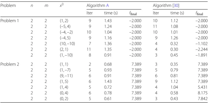
The numerical results in Table1indicate that AlgorithmAis much more robust than Algorithm [30], although the CPU time of AlgorithmAis more than that of Algorithm [30]. The less time of Algorithm [30] is due to the fact that Algorithm [30] only solves a subproblem at each iteration.

Table 1 Numerical results

Problem n m x0 _{AlgorithmA Algorithm [30]}

Iter time (s) ffinal Iter time (s) ffinal

Problem 1 2 2 (1, 2) 9 1.43 –2.000 10 1.12 –2.000

2 2 (–5, 4) 9 1.24 –2.000 11 1.08 –2.000

2 2 (–4, –2) 10 1.04 –2.000 10 1.01 –2.000

2 2 (–4, 5) 9 1.16 –2.000 9 1.26 –2.000

2 2 (10, –10) 7 1.36 –2.000 4 0.32 –1.102

2 2 (2, 1) 11 1.35 –2.000 4 0.30 –2.244

2 2 (1, –10) 8 0.91 –2.000 3 0.45 –1.891

Problem 2 2 2 (1, 1) 2 0.68 7.389 3 0.35 7.389

2 2 (1, –7) 5 0.93 7.389 5 0.79 7.389

2 2 (9, –11) 6 0.91 7.389 6 0.81 7.389

2 2 (1, 5) 6 1.43 7.389 9 1.12 7.389

2 2 (1, 4) 5 0.72 7.389 4 1.04 5.431

2 2 (0, 4) 6 0.78 7.389 4 0.58 8.175

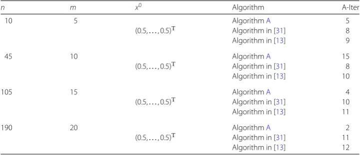
Table 2 Numerical results of NCM

n m x0 _{Algorithm A-Iter}

10 5 AlgorithmA 5

(0.5,. . ., 0.5)T _{Algorithm in [31] 8} Algorithm in [13] 9

45 10 AlgorithmA 15

(0.5,. . ., 0.5)T _{Algorithm in [31] 8} Algorithm in [13] 10

105 15 AlgorithmA 4

(0.5,. . ., 0.5)T Algorithm in [31] 10 Algorithm in [13] 11

190 20 AlgorithmA 2

(0.5,. . ., 0.5)T _{Algorithm in [31] 11} Algorithm in [13] 12

Problem 3([13]) The nearest correlation matrix (NCM) problem:

min f(X) =1

2X–C

2

F

s.t XI,

Xii= 1, i= 1, 2, . . . ,m,

(6.3)

whereC∈Sm_{is a given matrix,X∈S}m_{,is a scalar.}

In the implementation,= 10–3, the matrixCis generated randomly, and its diagonal elements are 1. We test ten times for every fixed dimensionality.

The numerical results are listed in Table2. The meaning of the notations in Table2is described as follows:

n: the dimensionality ofx; m: the order of the matrixA(x); A-Iter : the average iterative number.

The numerical results in Table2 indicate that the average iterative number of Algo-rithmAis less than that of the other two algorithms. Hence, AlgorithmAis comparable.

7 Concluding remarks

In this paper, we have presented a new SSDP algorithm for nonlinear semidefinite pro-gramming. Two subproblems, which are constructed skillfully, are solved to generate the master search directions. In order to avoid the Maratos effect, a second-order correction direction is introduced by solving a new quadratic programming. A penalty function is used as a merit function for arc search. The global convergence and superlinearly conver-gence of the proposed algorithm are shown under some mild conditions. The preliminary numerical results indicate that the proposed algorithm is effective and comparable.

Funding

The work is supported by the National Natural Science Foundation (No.11561005) and the Science Foundation of Guangxi Province (No. 2016GXNSFAA380248).

Availability of data and materials

Competing interests

The authors declare that they have no competing interests.

Authors’ contributions

The authors completed the paper. The authors read and approved the final manuscript.

Authors’ information

Jianling Li, Email: jianlingli@126.com; Hui Zhang, Email: 605007820@qq.com

Publisher’s Note

Springer Nature remains neutral with regard to jurisdictional claims in published maps and institutional affiliations.

Received: 19 March 2019 Accepted: 7 August 2019

References

1. Tuyen, N.V., Yao, J.C., Wen, C.F.: A note on approximate Karush–Kuhn–Tucker conditions in locally Lipschitz multiobjective optimization. Optim. Lett.13, 163–174 (2019)

2. Chang, S.S., Wen, C.F., Yao, J.C.: Common zero point for a finite family of inclusion problems of accretive mappings in Banach spaces. Optimization67, 1183–1196 (2018)

3. Takahashi, W., Wen, C.F., Yao, J.C.: The shrinking projection method for a finite family of demimetric mappings with variational inequality problems in a Hilbert space. Fixed Point Theory19, 407–419 (2018)

4. Kanno, Y., Takewaki, I.: Sequential semidefinite program for maximum robustness design of structures under load uncertainty. J. Optim. Theory Appl.130(2), 265–287 (2006)

5. Jarre, F.: An interior point method for semidefinite programming. Optim. Eng.1, 347–372 (2000)

6. Ben, T.A., Jarre, F., Kovara, M., Nemirovski, A., Zowe, J.: Optimization design of trusses under a nonconvex global buckling constraint. Optim. Eng.1, 189–213 (2000)

7. Noll, D., Torki, M., Apkarian, P.: Partially augmented Lagrangian method for matrix inequality constraints. SIAM J. Optim.15(1), 161–184 (2001)

8. Sun, J., Zhang, L.W., Wu, Y.: Properties of the augmented Lagrangian in nonlinear semidefinite optimization. J. Optim. Theory Appl.129(3), 437–456 (2006)

9. Sun, D.F., Sun, J., Zhang, L.W.: The rate of convergence of the augmented Lagrangian method for nonlinear semidefinite programming. Math. Program.114(2), 349–391 (2008)

10. Luo, H.Z., Wu, H.X., Chen, G.T.: On the convergence of augmented Lagrangian methods for nonlinear semidefinite programming. J. Glob. Optim.54(3), 599–618 (2012)

11. Wu, H.X., Luo, H.Z., Ding, X.D.: Global convergence of modified augmented Lagrangian methods for nonlinear semidefinite programming. Comput. Optim. Appl.56(3), 531–558 (2013)

12. Wu, H.X., Luo, H.Z., Yang, J.F.: Nonlinear separation approach for the augmented Lagrangian in nonlinear semidefinite programming. J. Glob. Optim.59(4), 695–727 (2014)

13. Yamashita, H., Yabe, H., Harada, K.: A primal-dual interior point method for nonlinear semidefinite programming. Math. Program.135, 89–121 (2012)

14. Yamashita, H., Yabe, H.: Local and superlinear convergence of a primal-dual interior point method for nonlinear semidefinite programming. Math. Program.132, 1–30 (2012)

15. Fares, B., Noll, D., Apkarian, P.: Robust control via sequential semidefinite programming. SIAM J. Control Optim.40, 1791–1820 (2002)

16. Correa, R., Ramirez, H.C.: A global algorithm for nonlinear semidefinite programming. SIAM J. Optim.15(1), 303–318 (2004)

17. Wang, Y., Zhang, S.W., Zhang, L.W.: A note on convergence analysis of an SQP-type method for nonlinear semidefinite programming. J. Inequal. Appl.2008, 218345 (2007)

18. Gomez, W., Ramirez, H.: A filter algorithm for nonlinear semidefinite programming. Appl. Math. Comput.29(29), 297–328 (2010)

19. Zhu, Z.B., Zhu, H.L.: A filter method for nonlinear semidefinite programming with global convergence. Acta Math. Sin. 30(10), 1810–1826 (2014)

20. Zhao, Q., Chen, Z.W.: On the superlinear local convergence of a penalty-free method for nonlinear semidefinite programming. J. Comput. Appl. Math.308, 1–19 (2016)

21. Zhao, Q., Chen, Z.W.: An SQP-type method with superlinear convergence for nonlinear semidefinite programming. Asia-Pac. J. Oper. Res.35, 1850009 (2018)

22. Zhang, J.L., Zhang, X.S.: A robust SQP method for optimization with inequality constraints. J. Comput. Appl. Math. 21(2), 247–256 (2003)

23. Theobald, C.M.: An inequality for the trace of the product of two symmetric matrices. Math. Proc. Camb. Philos. Soc. 77(2), 265–267 (1975)

24. So, W.: Commutativity and spectra of Hermitian matrices. Linear Algebra Appl.212–213(15), 121–129 (1994) 25. Dunn, J.C.: On the convergence of projected gradient processes to singular critical points. J. Optim. Theory Appl.

55(2), 203–216 (1987)

26. Burke, J.V., Moré, J.J.: On the identification of active constraints. SIAM J. Numer. Anal.25, 1197–1211 (1988) 27. Burke, J.V., Han, S.P.: A robust sequential quadratic programming method. Math. Program.43(1–3), 277–303 (1989) 28. Bonnans, J.F., Shapiro, A.: Perturbation Analysis of Optimization Problems, vol. 13, pp. 63–83. Springer, Berlin (2000) 29. Sun, D.F.: The strong second-order sufficient condition and constraint nondegeneracy in nonlinear semidefinite

programming and their implications. Math. Oper. Res.31(4), 761–776 (2006)

30. Li, Z.Y.: Differential-Algebraic Algorithm and Sequential Penalty Algorithm for Semidefinite Programming. Fujian Normal University, Fujian (2006) (in Chinese)