Approximate Closed Form Formulas for the Zeros of the Bessel Polynomials

Volume 2012, Article ID 873078,10pages doi:10.1155/2012/873078

Research Article

Approximate Closed-Form Formulas for

the Zeros of the Bessel Polynomials

Rafael G. Campos and Marisol L. Calder ´on

Facultad de Ciencias F´ısico-Matem´aticas, Universidad Michoacana, 58060 Morelia, MN, Mexico

Correspondence should be addressed to Rafael G. Campos,[email protected]

Received 11 June 2012; Revised 10 September 2012; Accepted 23 September 2012

Academic Editor: Stefan Samko

Copyrightq2012 R. G. Campos and M. L. Calder ´on. This is an open access article distributed under the Creative Commons Attribution License, which permits unrestricted use, distribution, and reproduction in any medium, provided the original work is properly cited.

We find approximate expressionsxk, n, aandyk, n, afor the real and imaginary parts of thekth zerozkxkiykof the Bessel polynomialynx;a. To obtain these closed-form formulas we use the fact that the points of well-defined curves in the complex plane are limit points of the zeros of the normalized Bessel polynomials. Thus, these zeros are first computed numerically through an implementation of the electrostatic interpretation formulas and then, a fit to the real and imaginary parts as functions ofk, n and a is obtained. It is shown that the resulting complex number

xk, n, a iyk, n, aisO1/n2_{-convergent toz}

kfor fixedk.

1. Introduction

The polynomial solutions of the differential equation

z2_{yz az2yz−nna−1yz 0, a >0, z∈C, 1.1}

were studied systematically in 1 by the first time. They are namedgeneralized Bessel polynomials and are given explicitly by

ynz;a n

k0

n!na−1_k n−k!k!

_z

2

k

, 1.2

written in terms of the polynomial solutions of1.1. Also, this equation has application in

network and filter design, isotropic turbulence fields, and moresee the monograph2or 3–14and references therein for some other results. Among these, several results about the

important problem concerning the location of its zeros have been obtained 8–11 and in 12, explicit expressions for sum rules and for the homogeneous product sum symmetric

functions of zeros of these polynomials are given. On the other hand, the electrostatic interpretation of these zeros as the equilibrium configuration in the complex plane with a logarithmic electric potential and a dipole at the origin has been given in13, and in14

it is shown that this equilibrium configuration is not stable. Thus, these cases show that it is desirable to acquire new analytical knowledge about the location of the zeros of the Bessel polynomials.

In this paper we give approximate explicit formulas for both the real and imaginary parts of thekth zerozkxkiykofynz;aand show that the approximation order of these

new formulas to the exact zeros of the Bessel polynomials isO1/n2_{for fixedk.}

The approach followed in this paper is simple and based on three items. The first is the electrostatic interpretation of the zeros of polynomials satisfying second-order differential equations15–17, the second is a simple curve fitting of numerical data, and the third is the

known fact that the points of well-defined curves in the complex plane are limit points of the zeros of the normalized Bessel polynomials8–11. The formulas yielded by the electrostatic

interpretation of the zeros of Bessel polynomials are used to find them numerically as it has been done previously with these and other sets of points 7–19. Several sets of zeros are

computed in this way and the sets of real and imaginary values are fitted by polynomials depending on the indexkwhose coefficients depend onnanda.

2. Asymptotic Expressions for the Zeros

Let zk xkiyk,k 1,2, . . . , n, be the zeros of the Bessel polynomial ynz;a, ordered

according to the imaginary part. Then, from1.1it follows thatA procedure for obtaining this kind of nonlinear equations for the zeros of a polynomial satisfying second and higher order differential equations is given in19.

n

k1

1

zj−zk

azj2

2z2 j

0, 2.1

where j 1,2, . . . , n, that is, the real and imaginary parts of the zeros should satisfy the electrostatic equations

n

k1

xj−xk

xj−xk2yj−yk2

ax

3

j2x2jaxjy2j −2yj2

2x2_jy2_j2

0,

n

k1

yj−yk

xj−xk2yj−yk2

yj

ax2

j4xjay2j

2x2

jy2j

2 0.

0 −1.5 −1 −0.5 ( z )

a=2

0

Re

200 300 400 500

k

a

0

Im

200 300 400 500

1

−0.5

−1

0 0.5

a=2

( z ) k b 0 −1 −0.6 −0.2 −0.4 −0.8 −1.2 −1.4 ( z )

a=40

0 100 200 300 400 500

k Re c 1 −0.5 −1 0 0.5 ( z )

a=40

0 100 200 300 400 500

k Im d 0 −1 −0.6 −0.2 −0.4 −0.8 −1.2 −1.4 ( z )

0 100 200 300 400 500

k

a=100

Re e 1 −0.5 −1 0 0.5 ( z )

0 100 200 300 400 500

k

a=100

Im

f

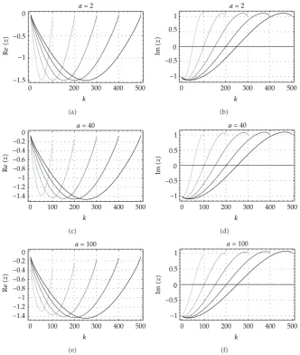
Figure 1: Real and imaginary parts of the zeros of the normalized Bessel polynomialsyn2z/2na−2;a

fora2,40,100. They are plotted as functions ofkforn100,200,300,400,500, in gray-level intensity, from lower to higher, according to the value ofn.

This set of nonlinear equations can be solved by standard methods. We have used a Newton method to solve them up ton500 anda100.

Letωkμkiνkbe thekth zero of the normalized Bessel polynomialsyn2z/2na−

2;a, that is,μk 2na−2xk/2 andνk 2na−2xk/2. As it is shown inFigure 1,

the piecewise linear interpolation of the real and imaginary parts of ωk can be fitted by

polynomials of the second and third degree in the indexk. Thus, we propose the following expressions

μk, n, a a2n, ak2a1n, aka0n, a,

νk, n, a b3n, ak3b2n, ak2b1n, akb0n,

0

−0.8

−0.6

−0.4

−0.2

0 100 200 300 400 500

n

∼

μ

(

1

,n

,a

)

a

0 100 200 300 400 500

n

−1.4

−1.5

−1.3

−1.2

−1.1

∼

μ

(

n/

2

,n

,a

)

b

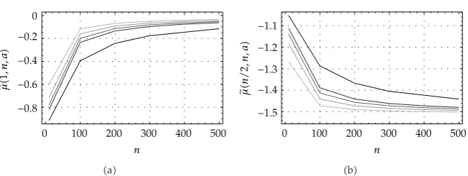
Figure 2: Dependence ofμ1, n, aandμn/2, n, aonnfora10,20,30,40,100. Plots are shown in gray-level intensity, from lower to higher, according to the value ofa.

for the approximate zeroω_kμk, n, a iνk, n, ato fit our data. To find the dependence of the coefficients of these polynomials onnanda, we take into account the numerical behavior of the data at the middle and end points.

We begin by finding the coefficients of the second-order polynomial giving the real part by fitting the values of μk, n, a at k 1 and k n/2. In Figure 2 we show the dependence ofμ1, n, aandμn/2, n, aonnfor some values ofa.

A fit of these data to the models−A/nBand−A/nB−3/2 yields

μ1, n, a − 54a860

100n50a715, μ

_n

2, n, a

−75n−2a400

50n11a220. 2.4

These conditions and the symmetry ofμk, n, awith respect to the middle point lead to the following coefficients:

a2n, a

p2n, a

rn, a, a1n, a

p1n, a

rn, a, a0n, a

p0n, a

rn, a, 2.5

where

p2n, a 4

7500n2_{50625n850an−694a}2_{−2770a96800,}

p1n, a −4n1

7500n250625n850an−694a2−2770a96800,

p0n, a −100

130n2−993n−7656

−20135n2627n−1580a−2297n794a2,

rn, a 5nn−250n11a22020n10a143.

2.6

Now, to find the coefficients of the third-order polynomial giving the imaginary part we follow a similar procedure. The dependence of the real part of ν1, n, a and ∂νk, n, a/

0 100 200 300 400 500

−1

−0.9

−0.8

−0.7

−0.6

−0.5

(

1

,n

,a

)

n

∼

ν

a

0 0.05 0.1 0.15 0.2 0.25

k

(

n/

2

,n

,a

)

0 100 200 300 400 500

n

∼

ν

b

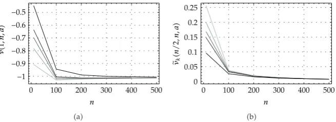
Figure 3: Dependence ofν1, n, aand∂νk, n, a/∂k|kn/2onnfora10,20,30,40,100. Plots are shown

in gray-level intensity, from lower to higher, according to the value ofa.

Again, a fit of these data to the modelsA/nB−1 andA/nyields

ν1, n, a −25₂₅n−_na₋−₁50, ∂νk, n, a_∂k

kn/2

96

na25. 2.7

In addition, we have that

νn

2, n,2

0, νn, n,2 −ν1, n,2, 2.8

therefore, the coefficients are given by

b3n, a

q3n, a

sn, a, b2n, a

q2n, a

sn, a,

b1n, a

q1n, a

sn, a, b0n, a

q0n, a

sn, a,

2.9

where

q3n, a −200

23n3−92n290n4200n3−5n28n−6a

−8n2−2n2a2,

q2n, a 100

69n4−255n3186n292n8

−1003n4−12n39n24n−12a43n3−3n24a2,

q1n, a 50

21n454n3−522n2748n−176

q0n, a −25

25n4_−217n3_618n2_−660n184

−25n4−2n3−7n216n−12an3n2−4n4a2

sn, a 25n−12_n−22_a25.

2.10

Thus, the substitution of2.10,2.9,2.6, and2.5, respectively, in2.3yields the approxi-mate closed-form expressions

zkxk, n, a iyk, n, a 2₂μ_nk, n, a_a−2i 2₂ν_nk, n, a_a−2, 2.11

where k 1,2, . . . , n, for the zeros of the unnormalized Bessel polynomial ynz;a. The

expressions given in2.11converge to the zeros zkof these polynomials, as we will show

in the following.

3. Convergence

Following9, we define

Wz e

√

11/z2

z1 11/z2, 3.1

and denote byΓthe curve defined by

Γ z∈C:|Wz|1, argz≥ π 2

, 3.2

which contains the limit points ωk of the zeros of the normalized Bessel polynomial

yn2z/2na−2;a. Then, it has been proved in8that the zeroωkofyn2z/2na−2;a

approaches to orderO1/nthe limit valueωk, that is,

|ωk−ωk|O

1

n

, 3.3

asn → ∞.

Thus, if we show that|ω_k−ω_k|O1/n, we will have proved that

|ωk−ωk|O

1

n

, 3.4

and therefore, taking into account thatωk 2na−2zk/2, the explicit expression2.11

approaches to orderO1/n2_{the zeroz}

To this purpose, we simply substitute the expression forωk μk, n, a iνk, n, a

given by2.3in3.1to obtain, after a lengthy calculation, that the expansion ofWω_kin terms of 1/nis

Wωk 1

2a2_{−100a3k−2−5042k−67}

25a25

₂₅h_ak, a₂₅cos2tk, a−sin2tk, a1

nO

1

n3/2

,

3.5

where

hk, a 25a2_13027a300k2_2a2_{−100a3k−2−5042k−67}2_,

tk, a 25a13027a300k

41675−100aa2_{−1050k150ak}.

3.6

This implies that

|Wωk|1O

1

n

, 3.7

for fixedkanda. Thus,ωkapproaches to orderO1/ntheΓcurve and3.4follows. From

here we have that

|zk−zk|O

1

n2

, 3.8

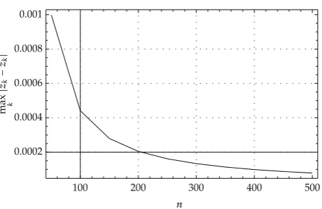
as n → ∞. Numerical calculations confirm and extend this result. Figure 4 shows the behavior of the maxima of|zk−zk|overkas they depend onnfor the particular case ofa2.

The numbers computed by2.2are taken as the exact zerosz_k. A fit of these data gives 1/na witha1.7.

4. Some Few Tests

Just to give examples of the application of the approximate expression2.11, we consider the

following cases.

4.1. The Real Zero

A closed-form formula for the unique real zeroα_naof the Bessel polynomialy_nz;acan be obtained by the substitution ofk n1/2 in the real part of2.11,xk, n. This gives

αna −4₃n₇₅1 50−71a

−707a2_5900a35000

7500n O

1

n2

100 200 300 400 500 0.0002

0.0004 0.0006 0.0008 0.001

max k

n

|

zk

−

∼

zk

|

Figure 4: Plot of the values of maxn

k1|zk−zk|againstnfor the case ofa2.

as our new result. In2,11very accurate expressions forα_naare given. Particularly, the following formula:

2

αna −1.325486838n−1.00628995a1.349836480O

1 2na−2

, 4.2

is given in11. Expanding 2/α_nain powers ofnwe find that

2

αna −1.33333n−0.946667a0.666667, 4.3

indicating good relative agreement between the two results.

4.2. Power Sums

Here we carry out the corresponding multiplications and use some cases of Faulhaber’s formula. Then we compare our results with the exact ones.

1Sum of the Zeros. The simple sum ofz_kcf.2.11gives a complicated expression

for the real part. However, expanding both the real and imaginary parts of this sum gives

s1n n

k1

zk−1

53a 100 −

71 30i

32

a25

1

nO

1

n2

. 4.4

The exact result iss1n −1, as can be seen from1.2.

2Sum of the Squares of the Zeros. In this case we take the particular case ofa1. For

this value we obtain

s2n n

k1

z2

k

3469 5915nO

1

n2

The exact sum

s2n

1 2n−1

1 2nO

1

n2

4.6

can be found elsewhere12.

The use of the approximate formula 2.11 for obtaining sums of higher powers of these zeros is not expected to give satisfactory results, since the powers and the sum magnify the total error.

5. Final Comment

The approximate formula forzkgiven above is far from being unique. There exist many other

functions to fit the zeros obtained through the electrostatic equations2.2, and there are other

conditions to impose at the extreme and middle points of the fitting interval. For instance, the imaginary partyk, ncan be fitted by a polynomial of degree 5, but this does not improve the rate of convergence and, on the other hand, the calculations become more complicated.

Acknowledgment

The authors thank Consejo Nacional de Ciencia y Tecnolog´ıa for the financial support given to this project.

References

1 H. L. Krall and O. Frink, “A new class of orthogonal polynomials: the Bessel polynomials,”

Trans-actions of the American Mathematical Society, vol. 65, pp. 100–115, 1949.

2 E. Grosswald, Bessel Polynomials, vol. 698 of Lecture Notes in Mathematics, Springer, Berlin, Germany, 1978.

3 H. M. Srivastava, “Some orthogonal polynomials representing the energy spectral functions for a family of isotropic turbulence fields,” Zeitschrift f ¨ur Angewandte Mathematik und Mechanik, vol. 64, no. 6, pp. 255–257, 1984.

4 J. L. L ´opez and N. M. Temme, “Large degree asymptotics of generalized Bessel polynomials,” Journal

of Mathematical Analysis and Applications, vol. 377, no. 1, pp. 30–42, 2011.

5 O. E ˘gecio ˘glu, “Bessel polynomials and the partial sums of the exponential series,” SIAM Journal on¨

Discrete Mathematics, vol. 24, no. 4, pp. 1753–1762, 2010.

6 C. Berg and C. Vignat, “Linearization coefficients of Bessel polynomials and properties of Student

t-distributions,” Constructive Approximation, vol. 27, no. 1, pp. 15–32, 2008.

7 L. Pasquini, “Accurate computation of the zeros of the generalized Bessel polynomials,” Numerische

Mathematik, vol. 86, no. 3, pp. 507–538, 2000.

8 A. J. Carpenter, “Asymptotics for the zeros of the generalized Bessel polynomials,” Numerische

Mathe-matik, vol. 62, no. 4, pp. 465–482, 1992.

9 F. W. J. Olver, “The asymptotic expansion of Bessel functions of large order,” Philosophical Transactions

of the Royal Society of London Series A, vol. 247, pp. 328–368, 1954.

10 H.-J. Runckel, “Zero-free parabolic regions for polynomials with complex coefficients,” Proceedings of

the American Mathematical Society, vol. 88, no. 2, pp. 299–304, 1983.

11 M. G. de Bruin, E. B. Saff, and R. S. Varga, “On the zeros of generalized Besselpolynomials I, II,”

Indagationes Mathematicae, vol. 84, pp. 1–25, 1981.

12 F. G´alvez and J. S. Dehesa, “Some open problems of generalised Bessel polynomials,” Journal of Physics

13 E. Hendriksen and H. van Rossum, “Electrostatic interpretation of zeros,” in Orthogonal Polynomials

and Their Applications, M. Alfaro, J. S. Dehesa, F. J. Marcellan, J. L. Rubio de Francia, and J. Vinuesa,

Eds., vol. 1329 of Lecture Notes in Mathematics, pp. 241–250, Springer, Berlin, Germany, 1988.

14 G. Valent and W. Van Assche, “The impact of Stieltjes’ work on continued fractions and orthogonal polynomials: additional material,” Journal of Computational and Applied Mathematics, vol. 65, no. 1–3, pp. 419–447, 1995.

15 G. Szeg˝o, Orthogonal Polynomials, Colloquium Publications, American Mathematical Society, Provi-dence, RI, USA, 1975.

16 F. Marcell´an, A. Mart´ınez-Finkelshtein, and P. Martinez-Gonzalez, “Electrostatic models for zeros of polynomials: old, new, and some open problems,” Journal of Computational and Applied Mathematics, vol. 207, pp. 258–272, 2007.

17 R. G. Campos, “Perturbed zeros of classical orthogonal polynomials,” Boletin de la Sociedad Matematica

Mexicana, vol. 5, no. 1, pp. 143–153, 1999.

18 R. G. Campos, “Solving singular nonlinear two-point boundary value problems,” Boletin de la Sociedad

Matematica Mexicana, vol. 3, no. 2, pp. 279–297, 1997.

Submit your manuscripts at

http://www.hindawi.com

Hindawi Publishing Corporation

http://www.hindawi.com Volume 2014

Mathematics

Hindawi Publishing Corporation

http://www.hindawi.com Volume 2014

Hindawi Publishing Corporation http://www.hindawi.com

Differential Equations

International Journal of

Volume 2014

Applied MathematicsJournal of

Hindawi Publishing Corporation

http://www.hindawi.com Volume 2014

Hindawi Publishing Corporation

http://www.hindawi.com Volume 2014

Hindawi Publishing Corporation

http://www.hindawi.com Volume 2014

Mathematical PhysicsAdvances in

Complex Analysis

Hindawi Publishing Corporation

http://www.hindawi.com Volume 2014

Optimization

http://www.hindawi.com Volume 2014

Combinatorics

Hindawi Publishing Corporation

http://www.hindawi.com Volume 2014

International Journal of

Hindawi Publishing Corporation

http://www.hindawi.com Volume 2014

Journal of

Hindawi Publishing Corporation

http://www.hindawi.com Volume 2014

Function Spaces

Abstract and Applied Analysis

Hindawi Publishing Corporation

http://www.hindawi.com Volume 2014

International Journal of Mathematics and Mathematical Sciences

Hindawi Publishing Corporation http://www.hindawi.com Volume 2014

The Scientific

World Journal

Hindawi Publishing Corporation

http://www.hindawi.com Volume 2014

Hindawi Publishing Corporation

http://www.hindawi.com Volume 2014

Discrete Dynamics in Nature and Society

Hindawi Publishing Corporation

http://www.hindawi.com Volume 2014

Hindawi Publishing Corporation

http://www.hindawi.com Volume 2014

Discrete Mathematics

Hindawi Publishing Corporation

http://www.hindawi.com Volume 2014

Hindawi Publishing Corporation