2018 IX International Conference on Optimization and Applications (OPTIMA 2018) ISBN: 978-1-60595-587-2
Branch and Bound Algorithm for the Single Machine Scheduling Problem
with Release and Delivery times
Natalia GRIGOREVA
St. Petersburg State University Universitetskaja nab. 7/9, 199034 St. Petersburg, Russia
Keywords: Single processor, Branch and bound algorithm, Inserted idle time.
Abstract. The single machine scheduling problem is one of the classic NP-hard optimization
problems, and it is useful in solving flowshop and jobshop scheduling problems. The goal of this paper is to prepare algorithms for the scheduling problem, where set of tasks is performed on a single processor. Each task has a release time when it becomes available for processing, a processing time and a delivery time. At most one job can be processed at a time, but all jobs may be simultaneously delivered. Preemption is not allowed. The objective is to minimize the time, by which all tasks are delivered. We compare the nondelay schedule, in which no processor is kept idle at a time when it could begin processing a task and an inserted idle time schedule, in which a processor is kept idle at this time.
In this paper, we propose an approximation algorithm and by combining this algorithm and branch and bound method, we develop branch and bound algorithm, which can find optimal solutions for the single processor scheduling problem. We use a binary branching rule, where at each branch node, a complete schedule is generated.
To illustrate the effectiveness of our algorithms we tested them on randomly generated set of tasks.
Introduction and Related Work
This paper is concerned with a single machine scheduling problem of minimizing the makespan. Following the 3-field classification scheme proposed by Graham et al. [9], the problem under
consideration is denoted by 1|rj, qj|Cmax. The problem relates to the scheduling problem [5] and
has many applications. Lenstra in [14] showed that the problem is NP -hard in the strong sense. We consider a system of tasks U = {u1, u2, . . . , un}. Each task is characterized by its execution
time t(ui), its release time (or head) r(ui) and its delivery time (or tail) q(ui). Release time r(ui) is the time at which the task is ready to start processing, and its delivery begins immediately after processing has been completed. The delivery time is equal q(ui). At most one job can be processed
at a time, but all jobs may be simultaneously delivered. The set of tasks is performed on a single processor. Task preemption is not allowed. The schedule defines the start time τ(ui) of each task ui∈ U. The makespan of the schedule S is the quantity
Cmax = max{τ(ui) + t(ui) + q(ui)|ui∈ U}.
The objective is to minimize Cmax, the time by which all jobs are delivered.
The problem is equivalent to model 1|rj|Lmax with release times and due dates, rather than delivery times. In this problem, the objective is to minimize the maximum lateness of jobs. The equivalence is shown by replacing each delivery time q(ui) by due dated(ui) = qmax−q(ui),where qmax = max{q(ui) | ui ∈ U}. The 1|rj, qj|Cmax is also a key component of several more complex scheduling problems. Problem is useful in solving flowshop and jobshop scheduling problems [1, 2, 7] and plays a central role in some real industrial application [20].
The approximation algorithms for the single processor scheduling problem were given by Potts [19], Hall and Shmoys [12], Nowicki and Smutnicki [17].
The above algorithms used extended Jackson’s rule with some modifications. The problem is solved by the extended Jackson’s rule: whenever the machine is free and one or more tasks available for processing, schedule an available task with the earliest due data. Potts proposed anO(n2log(n)) iterated algorithm, which generated nschedules and selected the best one. Nowicki and Smutnicki [17] presented a more efficient 3/2 approximation algorithm which runs in O(nlog(n)). Hall and Shmoys improved Potts algorithm when applied it to both the original and reversed problems (in which the release date and delivery times are reversed). The worst-case performance ratio of there algorithm is equal 4/3.
The works of Baker and Su [4], McMahon and Florian[16], Carlier [6], Grabowski et al. [8] and Pan and Shi [18] developed branch and bound algorithms to solve the given problem using different branching rules and bounding techniques. The most efficient algorithm is algorithm by Carlier, which optimally solves instances with up to thousands of jobs. This algorithm constructs a full solution in each node of the search tree. Liu [15] modified Carlier algorithm to solve the problem with precedence constraints very efficiently. Chandra et al. [7] developed a branch and bound algorithm to solve the problem 1|rj, prec|fmax, the problem under consideration is the special case of this problem.
In fact, most heuristic algorithms can construct a nondelay schedule, which was defined by Baker [2] as a feasible schedule, with no processor being kept idle at the time when it could begin processing a task. An inserted idle time schedule (IIT) was defined by Kanet and Sridharam in [13] as a feasible schedule in which a processor is kept idle at the time when it could begin processing a task. Kanet and Sridharam [13] reviewed the literature on the problem setting that can require IIT scheduling.
We are interested in developing the inserted idle time algorithms for some scheduling prob-lems. In [10] we considered scheduling with inserted idle time for m parallel identical processors and proposed the branch and bound algorithm for the multiprocessor scheduling problem with precedence-constrained tasks. In [11] we proposed the approximation IIT algorithm forP|rj|Lmax problem. The aim of the paper is to present IIT schedule for 1|rj, qj|Cmax problem.
In this paper, we propose an approximation IIT algorithm named IJR (idle Jackson’s rule). Then, by combining the IJR algorithm and B&B method, we develop BBI algorithm, which can find optimal solutions for the single processor scheduling problem. We use a binary branching rule, where at each branch node a complete schedule is generated.
This paper is organized as follows. The approximation algorithm IJR is presented in section 1. In section 2 we consider several properties of schedules, constructed by IJR algorithm, which help to recognize optimality of schedules and to obtain its lower bound. A branch and bound algorithm is described in details in section 3. Computational studies of the branch and bound algorithm are provided in section 4. Section 5 contains a summary of this paper.
Approximation Algorithm IJR
Algorithm IJR generates the schedule, in which processor is kept idle at the time when it could begin processing a job. The approximation schedule S is constructed by IJR algorithm as follows. Let rmin = min{r(i) | i ∈ U}, qmin = min{q(i) | i ∈ U}. Define the lower bound LB of the minimum makespan [6]:
LB = max{rmin+
n
X
i=1
t(i) +qmin,max{r(i) +t(i) +q(i)| i∈U}}.
Let k tasks have been put in the schedule and the partial schedule Sk has been constructed.
Lettimebe the time, when the processor finishes performing all jobs from the partial scheduleSk.
Then time:= max{τ(i) +t(i) |i∈Sk}.
1. If there is no job ui, such as r(ui)≤time, then time:= min{r(ui) | i /∈Sk}
Select the ready job u with maximum delivery time
q(u) = max{q(ui) | r(ui)≤time}.
2. Select jobu∗ with maximum delivery time, such as
q(u∗) = max{q(ui)| time < r(ui)< time+t(u)}.
3. If there is no such job u∗ or one of inequality is hold
q(u)≥q(u∗) or q(u∗)≤LB/3,
then we map jobv =u to the processor. Go to 11.
4. Define the idle time of the processor before the start of jobu∗ idle(u∗) =r(u∗)−time.
5. Ifq(u∗)−q(u)> idle(u∗), then we map job v =u to the processor. Go to 11. 6. Select jobu1 with maximum delivery time, such as
q(u1) = max{q(ui)| time≥r(ui) & t(ui)≤idle(u∗)}.
7. If we findu1, then we map v =u1 to the processor. Go to 11. 8. Select jobu2 with maximum delivery time, such as
q(u2) = max{q(ui)| time < r(ui) & r(ui) +t(ui)≤r(u∗)}.
9. If we findu2, then we map v =u2 to the processor. Go to 11. 10. We map the job v =u∗ to the processor.
11. Define the start time of job v: τ(v) := max{time, r(v)};
time:=τ(v) +t(v).
12. k :=k+ 1. Ifk < n, then go to 1.
We construct the approximation schedule S=Sn and find the objective function Cmax(S) = max{τ(ui) +t(ui) +q(ui)| ui ∈U}.
The algorithm sets on the processor the job u∗ with the large delivery time q(u∗). If this job is not ready, then the processor will be idle in the interval [t1, t2], where t1 =time, t2 =r(u∗). In order to avoid too much idle of the processor the inequality q(u∗)−q(u)≤idle(u∗) is verified on step 5. If the inequality is hold, we choose job u∗. In order to use the idle time of the processor we select job u1 or u2 to perform in this interval. Job u∗ starts atτ(u∗) =r(u∗).
To illustrate IJR heuristic we consider the Example 1. Let us consider the two-task problem with r1 = 0;t1 = T −1;q1 = 0;r2 = δ;t2 = 1;q2 = T −1. Then, IJR algorithm schedules the task 2 first, and the makespan of this schedule is equal toT + 1 +δ. IJR algorithm generates the
optimal schedule. The problem can be solved using extended Jackson’s rule (EJR): whenever the machine is free and one or more tasks are available for processing, schedule an available task with the greatest delivery time. For Example 1 extended Jackson’s rule (EJR) schedules the large task first, then the makespanCmax(EJ R) = 2T.
Properties of IIT Schedule S
We consider the properties of the schedules, constructed by the algorithm IJR.
Let algorithm generates a schedule S, then for each job j we have the start time τ(j). The objective function is Cmax(S) = max{τ(j) +t(j) +q(j) | j ∈U}.
We define critical job, critical sequence and interference job [19]. The definition of the delayed job is the new definition.
Definition 1. Critical job jc is the first processed job such as Cmax(S) =τ(jc) +t(jc) +q(jc). The delivery of critical job is completed last. Obviously, to reduce the objective function, the critical job must be started earlier.
Definition 2. Critical sequence in scheduleS is the sequence
J(S) = (ja, ja+1, . . . , jc), such as jc is the critical job and job ja is the earliest-scheduled job so
that there is no idle time between the processing of jobsja and jc.
The job ja is the first job in the schedule or there is any idle time before its beginning.
Definition 3.The job ju in a critical sequenceJ(S) is called the interference job, if q(ju)< q(jc)
and q(ji)≥q(jc) for i > u.
Lemma 1.If every jobji in the critical sequence satisfiesr(ji)≥r(ja) and q(ji)≥q(jc),then the
schedule S is optimal [19].
Now we define the delayed job, which can be started before a critical sequence.
Definition 4. The job jv in a critical sequence is called the delayed job if r(jv)< r(ja).
A interference job can be a delayed job too. LetCopt be the length of an optimal schedule. The
next Lemma bounds deviation of Cmax(S) from the optimum Copt.
Lemma 2. Let S be a schedule generated by IJR algorithm and Cmax(S) be the length of the scheduleS. Suppose thatju is the interference job for the critical sequence, thenCopt ≥Cmax(S)−
t(ju) +δ(S), where δ(S)>0.
Proof. Let T(J(S)) be the total processing time of jobs from the critical sequence T(J(S)) = Pc
i=at(ji), then
Cmax(S) =r(ja) +T(J(S)) +q(jc).
If there is interference job ju in the critical sequence, then we can represent the critical sequence
as J(S) = (S1, ju, S2), where S1 sequence jobs before ju, and S2 sequence jobs after ju. Let T(S1) = Pi∈S1t(ji). All jobs fromS2 are not available for processing at time t1 =r(ja) +T(S1). Letrmin(S2) = min{r(ji)|ji ∈S2}, then t1 < rmin(S2).
For an optimal schedule it is true:
Copt ≥rmin(S2) +T(S2) +q(jc),
then
Cmax(S)−Copt ≤r(ja) +T(J(S)) +q(jc)−rmin(S2)−T(S2)−q(jc) =
=r(ja) +T(S1) +t(ju)−rmin(S2) = t(ju)−δ(S).
Where δ(S) = rmin(S2)−t1. Then, we obtain Copt ≥Cmax(S)−t(ju) +δ(S).
This lemma refines the inequality, proved in [19] and shows how it is possible to improve the value of the objective function by removing the interference job from the critical sequence.
Our next lemma states result, which can eliminate some nodes from the search tree. Let S be a schedule generated by IJR algorithm and Cmax(S) be the length of the schedule S for problem
P.
Lemma 3. Let ju be the interference job for the critical sequence.
1. Consider new problem P L: constraint that the critical job precedes the interference job is added to problem P. Let Copt(P L) be the optimal makespan for problem P L. If the condition δ(S) ≥ q(jc)−q(ju) hold, then Cmax(S) ≤ Copt(P L). If the condition δ(S) < q(jc)−q(ju) hold,
then Copt≥Cmax(S) +δ(S)−q(jc) +q(ju)
2. Consider new problem P R: constraint that the interference job precedes S2 sequence is added. ThenCopt(P L)≥Cmax(S)−r(ja)−T(S1) +r(ju).
Proof. 1. Ifju is the interference job for the critical sequenceJ(S), thenCopt ≥Cmax(S)−t(ju) +
δ(S) by lemma 1.
Then at timet1 =r(ja)+T(S1) there are no any ready jobs in the sequenceS2andt1 < rmin(S2). If constraint that the critical job precedes the interference job is added, then
Copt(P L)≥rmin(S2) +T(S2) +t(ju) +q(ju),
Then
Cmax(S)−Copt(P L)≤r(ja) +T(J(S)) +q(jc)−rmin(S2)−T(S2)−t(ju)−q(ju) =
=r(ja) +T(S1)−rmin(S2) +q(jc)−q(ju) = −δ(S) +q(jc)−q(ju).
Where δ(S) = rmin(S2)−t1. If δ(S)≥q(jc)−q(ju) then
Cmax(S)≤Copt(P L) else Copt ≥Cmax(S) +δ(S)−q(jc) +q(ju).
2. If the interference job ju precedes S2 sequence, then
Copt(P R)≥r(ju) +t(ju) +T(S2) +q(jc).
Cmax(S)−Copt(P R)≤r(ja) +T(J(S)) +q(jc)−r(ju)−t(ju)−T(S2)−q(jc) =
=r(ja) +T(S1)−r(ju).
Then Cmax(S)−r(ja)−T(S1) +r(ju)≤Copt(P L).
Next lemma defines a lower bound for the node of the search tree if there is no interference job for the critical sequence, but there is the delayed job.
Lemma 4. Suppose that there is no interference job for the critical sequence, but there is the delayed job jv.
1. Consider new problem P L: constraint that the delayed jobjv precedes the critical sequence
is added. Then Copt(P L)≥Cmax(S)−r(ja) +r(jv).
2. Consider new problem P R: constraint that the first job ja of the critical sequence precedes
the delayed job jv is added. Let J1 ={ji ∈J(S)| r(ji)≥r(ja)} and T(J1) = P
i∈J2t(ji).
Then Cmax(S)−T(J(S)) +t(jv) +T(J1)≤Copt(P L).
Proof. 1. If the delayed job jv precedes the critical sequence, then
Copt≥r(jv) +T(J(S)) +q(jc).
Then
Cmax(S)−Copt(P R))≤r(ja) +T(J(S)) +q(jc)−r(jv)−T(J(S))−q(jc) =r(ja)−r(jv). Copt(P L)≥Cmax(S)−r(ja) +r(jv).
2. Let job ja of the critical sequence precedes the delayed job jv and J1 ={ji ∈J(S) | r(ji)≥ r(ja)}, then
Copt(P R)≥r(ja) +t(jv) +T(J1) +q(jc).
Cmax(S)−Copt(P R)≤r(ja) +T(J(S)) +q(jc)−r(ja)−t(jv)−T(J1)−q(jc) =
=T(J(S))−t(jv)−T(J1). Then Cmax(S)−T(J(S)) +t(jv) +T(J1)≤Copt(P L).
Branch and Bound Algorithm for Single Machine Scheduling Problem
The branch and bound algorithm is based on IJR algorithm, critical sequence, interference, and delayed jobs. Now we consider how to define a lower bound for the optimal solution. In section 1 we define two simple lower bounds for the makespan of the optimal scheduleCopt. We can compute the best lower bound by a preemptive algorithm. The preemptive problem 1|rj, qj, prmp|Cmax can be solved in O(n2) time [3]. The makespan of an optimum preemptive schedule is used as a lower bound for single machine scheduling problem by many researchers [4, 6, 7]. We apply the Baker algorithm [4] for computing the lower bound of the optimal solution. For most randomly generated instances tested in our paper the makespan of an optimum preemptive schedule is very close to the makespan of an optimum schedule.
Search tree. We construct a schedule S in every node of the tree. The upper boundU B is the value of the best solution known so far.
Branching. We apply the IJR algorithm to the single machine problem and construct the schedule S with objective function Cmax(S). Then we analyze the critical sequence J(S). If there are no interference job and any delayed job, then the schedule S is optimal.
If there is the interference job ju, then we can improve the lower bound LB(S) = Cmax(S)−
t(ju) +δ(S).
We define the critical sequence J(S) as J(S) = (S1, ju, S2) and consider two new problem. In the first problem we require job ju to be processed after all jobs of S2 by setting r(ju) =
max{r(jc) +t(jc), rmin(S2) +T(S2)}. In the second problem we require job ju to be processed
before all jobs of S2 by setting q(ju) = max{q(ju), q(jc) +T(S2)}.
If there is no interference job, but there is the delayed job jv, then we consider two new
problems too. In the first problem we require job jv to be processed before all jobs of J(S) by
setting q(jv) = q(ja). In the second problem we require job ju to be processed after job ja by
setting r(jv) =r(ja) +t(ja).
Now we formally describe our branch and bound algorithm, namely algorithmBBI, as follows: Step 1. Root node.
Step 1.1. Lower bound. Find a preemptive optimal schedule Sp by the Baker algorithm and
denote LB its makespan. If no job is preempted, then the schedule Sp is optimal for the root node
and the algorithm ends.
Step 1.2. Find a schedule S by IJR algorithm and denote Cmax(S) its makespan.
LetU B =Cmax(S). If LB =U B, then the schedule S is optimal and the algorithm ended. Step 1.3. Branch. Find critical sequence J(S). If there are no interference job and delayed jobs, then the schedule S is optimal and the algorithm ended.
Step 1.3.1. If there is the interference job ju in J(S), then we updateLB such as
LB = max(LB, Cmax(S)−t(ju) +δ(S)). IfLB ≥U B, then the current node cannot improve U B
and it is eliminated, else branch to a left and a right node as follows:
Left node. In the left node job ju is moved after critical job jc and a precedence constraint jc ≺ju is added. UpdateLB such as LB =max(LB, Cmax(S)−δ(S) +q(jc)−q(ju)).
If LB ≥U B, then the current node cannot improve U B and it is eliminated.
Right node. If the right node jobj(u) is moved before sequenceS2 and a precedence constraint
ju ≺S2 added. Update LB such as LB =max(LB, Cmax(S)−r(ja)−T(S1) +r(ju)).
If LB ≥U B, then the current node cannot improve U B and it is eliminated.
Step 1.3.2. If there is no an interference job, but there is the delayed job jv inJ(S), we update LB such as LB =max(LB, Cmax(S)−r(jv) +r(ja)).
If LB ≥U B,then the current node cannot improveU B and it is eliminated. Else branch to a left and a right node as follows:
Left node. In the left node job jv is moved before the critical sequence J(S) and a precedence
constraint jv ≺ja is added. UpdateLB such as LB =max(LB, Cmax(S)−r(ja) +r(jv)).
If LB ≥U B, then the current node cannot improve U B and it is eliminated.
Right node. If the right node jobjv is moved after the jobjaand a precedence constrainja≺jv
added. Update LB such as LB =max(LB, Cmax(S)−T(J(S) +t(jv) +T(J1)). If LB ≥U B, then the current node cannot improve U B and it is eliminated. Step 2. Nonroot node branch.
Step 2.1 Lower bound. If the newly added a precedence constraint is satisfied by the optimal preemptive schedule of the current node is the same as that of the father node, then lower bound of the current node is equal the lower bound of the father node; otherwise, we generate a preemptive optimal schedule Sp and find LB(S).
IfLB(S)≥U B,then the current node is eliminated. If no job is preempted, then the schedule is optimal for the current node, and we can update the upper bound U B = min(U B, Cmax(S)) and eliminate the current node.
Step 2.2 Upper bound. Find a schedule S by IJR algorithm and denote Cmax(S) its makespan. LetU B =Cmax(S). If LB =U B,then the schedule S is optimal and the algorithm ended.
Step 2.3 Binary branch.
If the optimal schedule is found for the current node, then the current node is eliminated else the schedule at the current node is branched as in step 1.3.
Computational Results
To illustrate the efficiency of our approach we tested it on randomly generated instances. We conduct computational studies over sets of random instances and compare the BBI algo-rithm with the Carlier algoalgo-rithm. The program for the algoalgo-rithm is coded in Object Pascal and compiled with Delphi 7. All the computational experiments were carried out on a laptop computer 1.9 GHz speed and 4 GB memory.
Three groups of instances were generated with discrete uniform distribution in a similar fashion than in [6]. The number of jobs considered is from n = 50 to n = 5000. Job processing time is generated with discrete uniform distributions between 1 and tmax. Release dates and delivery times are generated with discrete uniform distributions between 1 and Kn for K from 10 to 25. Parameter K controls the range of heads and tails. Job processing time was chosen with discrete uniform distributions from the following intervals:
1. t(j) from [1, tmax],
2. t(j) from [1, tmax/2], for j ∈1 :n−1 and t(jn) from [ntmax/8,3ntmax/8],
3. t(j) from [1, tmax/3], for j ∈1 :n−2 and t(jn−1), t(jn) from [ntmax/12,3ntmax/12]. Groups 2 and 3 contains instances with single long job and two long jobs.
Carlier [6] reported about a test set of 1000 instances, but he pointed out that the large majority of those instances was easy. Pan found [18] that most hard ones occur whenn= 100 and 14≤K ≤18.
For eachnandK = 20 we generate 100 instances and forn = 100 and forK between 10 and 25 we generate 100 instances too, i.e., a total of 1500 instances from group 1 are tested. We generate 100 instances for n = 100 and for K between 10 and 25 for group 2 and 3. The computational results are summarized in Tables 1—3.
The first column of this table contains the number of tasksn. For the BBI algorithm, columns
N V,N V M,N V T contains mean number of the search tree nodes, maximum number of the search tree nodes and mean computing time (in sec), respectively. For the Carlier algorithm columns
N V C,N V M C,N V T C contains mean number of the search tree nodes, maximum number of tree nodes and mean computing time. Table 1 shows the performance of the BBI algorithm and the Carlier algorithm according to the variation of the number of jobs for group 1. Parameter K = 20 and tmax= 50 for all instances in Table 1.
From this table we observe that average computing time and mean number of the search tree nodes increases with n for the Carlier algorithm. Mean number of the nodes does not increase with n and average computing time increases with n at a slow speed for algorithm BBI.
Table 2 shows the impact of the degree of the similarity in release times and delivery times on the effectiveness of two algorithms for group 1. Parameter K strongly affected the difficulty of the instances for the problem under consideration. Carlier [6] found that the most difficult instances take place when K=18,19,20. Chandra [7] noted that most challenging instances occur when K is
Table 1. Performance of algorithms according to the variation ofn.
n N V N V C N V M N V M C N V T N V T C
50 1.05 10.7 2 17 0.000 0.000
100 1.00 15.85 1 28 0.000 0.005
300 1.06 28.4 2 188 0.000 0.077
500 1.15 46.2 2 115 0.012 0.353
1000 1.05 52.5 2 220 0.047 1.792
2000 1.1 34.0 2 77 0.204 5.149
5000 1.05 59.4 2 146 1.381 72.843
Table 2. Performance of algorithms according to the variation ofK.
n K N V N V C N V M N V CM N V T N V T C
100 10 1.000 15.85 2 26 0.000 0.005
100 14 1.000 24.7 2 43 0.000 0.006
100 15 1.044 23.9 2 41 0.000 0.007.
100 16 1.000 21.45 2 44 0.000 0.008
100 18 1.000 20.65 2 42 0.000 0.006
100 20 1.000 15.85 1 28 0.000 0.005
100 22 1.050 13.12 2 26 0.000 0.004
100 25 1.000 7.6 1 18 0.000 0.004
between 10 and 25. Pan [18] found that most hard ones occur when n = 100 and 14 ≤K ≤ 18. We restricted our attention to these parameter ranges.
Mean number of the search tree nodes accepts the largest values at K between 14 and 18 for the Carlier algorithm. Mean number of the nodes does not change withK for theBBI algorithm. The BBI algorithm performs better than the Carlier algorithm in finding an optimal schedule with fewer branch nodes for instances from the group 1. The results for instances from the groups 2 and 3 are similar. So, we show in table 3 performance of two algorithms for group 2.
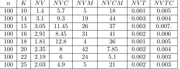
For instances from the group 2 the algorithm BBI generates more nodes of search tree on the average then for instances from the group 1. The maximum number of nodes is also increased. The Carlier algorithm generates fewer nodes on the average for instances from group 2 then from group 1. But, nevertheless, results of the algorithm BBI are better than those of the Carlier algorithm.
Table 3. Performance of algorithms according to the variation of K for the group 2.
n K N V N V C N V M N V CM N V T N V T C
100 10 1.4 5.7 5 18 0.001 0.005
100 14 3.1 9.3 19 44 0.003 0.004
100 15 3.05 11.45 26 37 0.003 0.007.
100 16 2.91 8.45 31 41 0.002 0.006
100 18 1.81 12.8 4 36 0.001 0.005
100 20 2.35 8 42 7.85 0.002 0.004
100 22 2.19 6 24 5.1 0.002 0.003
100 25 2.03 4.9 5 21 0.002 0.003
Our computational studies show that algorithm BBI reduces equally the number of search nodes and the computational time.
Conclusions
In this paper we investigated Inserted Idle Time schedules for 1|rj, qj|Cmax problem. We pro-posed an approximation IIT algorithm named as IJR and the branch and bound algorithm, which produces an optimal solution. The BBI algorithm is based on the IJR algorithm, uses a binary branching technique and a preemptive schedule to define a low bound. Algorithm BBI finds optimal solutions for all instances tested with up to 5000 jobs, which are randomly generated.
References
[1] C. Artigues and D. Feillet. A branch and bound method for the job-shop problem with sequence-dependent setup times, Annals of Operations Research. 159 (2008) 135-159.
[2] K.R. Baker. Introduction to Sequencing and Scheduling. John Wiley & Son, New York (1974). [3] K.R. Baker, E.L. Lawner, J.A. Lenstra, and A.H.G. Rinnooy Kan. Preemptive scheduling of a single machine to minimize maximum cost subject to release dates and precedence constrains, Operations Research. 31 (1983) 381-386.
[4] K.R. Baker and Z. Su. Sequensing with due-dates and early start times to minimize maximum tardiness, Naval Research Logistics Quarterly. 21 (1974) 171-176.
[5] P. Brucker. Scheduling Algorithms. fifth ed. Springer,Berlin (2007).
[6] J. Carlier. The one machine sequencing problem, European Journal of Operational Research. 11 (1982) 42-47.
[7] C. Chandra, Z. Liu, J. He, and T. Ruohonen. A binary branch and bound algorithm to minimize maximum scheduling cost, Omega. 42 (2014) 9-15.
[8] J. Grabowski, E. Nowicki, and S. Zdrzalka. A block approach for single-mashine scheduling with release dates and due dates, European Journal of Operational Research. 26 (1986) 278— 285.
[9] R.L. Graham, E.L. Lawner, and A.H.G. Rinnoy Kan. Optimization and approximation in deterministic sequencing and scheduling. A survey, Annals of Discrete Mathematics. 5 (10) (1979) 287-326.
[10] N.S. Grigoreva. Branch and bound method for scheduling precedence constrained tasks on parallel identical processors. Lecture Notes in Engineering and Computer Science: In proc. of The World Congress on Engineering 2014, London, U.K. (2014) 832-836,.
[11] N.S. Grigoreva. Multiprocessor Scheduling with Inserted Idle Time to Minimize the Maximum Lateness, In proceedings of the 7th Multidisciplinary International Conference of Scheduling: Theory and Applications. Prague, MISTA (2015) 814-816,.
[12] L.A. Hall and D.B. Shmoys. Jackson’s rule for single-machine scheduling: making a good heuristic better, Mathematics of Operations Research. 17 (1) (1992) 22-35.
[13] J. Kanet and V. Sridharan. Scheduling with inserted idle time:problem taxonomy and litera-ture review, Operations Research. 48 (1) (2000) 99-110.
[14] J.A. Lenstra, A.H.G. Rinnooy Kan, and P. Brucker. Complexity of machine scheduling prob-lems, Annals of Discrete Mathematics. 1 (1977) 343-362.
[15] Z. Liu. Single machine scheduling to minimize maximum lateness subject to release dates and precedence constraints, Computers & Operations Research. 37 (2010) 1537-1543.
[16] G.B. McMahon and N. Florian. On scheduling with ready times and due dates to minimize maximum lateness, Operations Research. 23 (3) (1975) 475-482.
[17] E. Nowicki and C. Smutnicki. An approximation algorithm for a single-machine scheduling problem with release times and delivery times, Discrete Applied Mathematics. 48 (1994) 69-79. [18] Y. Pan and L. Shi. Branch and bound algorithm for solving hard instances of the one-mashine
sequencing problem, European Journal of Operational Research. 168 (2006) 1030-1039. [19] C.N. Potts. Analysis of a heuristic for one machine sequencing with release dates and delivery
times, Operational Research. 28 (6) (1980) 445-462.
[20] K. Sourirajan and R. Uzsoy. Hybrid decomposition heuristics for solving large-scale scheduling problems in semiconductor wafer fabrication, Jornal of Scheduling. 10 (2007) 41-65.