M E T H O D O L O G Y A R T I C L E
Open Access
A proximity-based graph clustering
method for the identification and application
of transcription factor clusters
Maxwell Spadafore
1*, Kayvan Najarian
2,3and Alan P. Boyle
2,4Abstract
Background: Transcription factors (TFs) form a complex regulatory network within the cell that is crucial to cell functioning and human health. While methods to establish where a TF binds to DNA are well established, these methods provide no information describing how TFs interact with one another when they do bind. TFs tend to bind the genome in clusters, and current methods to identify these clusters are either limited in scope, unable to detect relationships beyond motif similarity, or not applied to TF-TF interactions.
Methods: Here, we present a proximity-based graph clustering approach to identify TF clusters using either ChIP-seq or motif search data. We use TF co-occurrence to construct a filtered, normalized adjacency matrix and use the Markov Clustering Algorithm to partition the graph while maintaining TF-cluster and cluster-cluster interactions. We then apply our graph structure beyond clustering, using it to increase the accuracy of motif-based TFBS searching for an example TF.
Results: We show that our method produces small, manageable clusters that encapsulate many known,
experimentally validated transcription factor interactions and that our method is capable of capturing interactions that motif similarity methods might miss. Our graph structure is able to significantly increase the accuracy of motif TFBS searching, demonstrating that the TF-TF connections within the graph correlate with biological TF-TF interactions. Conclusion: The interactions identified by our method correspond to biological reality and allow for fast exploration of TF clustering and regulatory dynamics.
Keywords: Transcription factors, Graph theory, Graph clustering, Network analysis, TF clusters, Genome regulation
Background
Transcription factors (TFs) are proteins that specifically regulate the transcription of DNA to RNA within the cell. There are an estimated 1300 human TFs, and they can act as suppressors or enhancers of transcription in a vari-ety of ways, either directly, by binding and remodeling the structure of DNA itself, or indirectly, by binding to and influencing other TFs [1]. The transcriptional regu-lation brought about by TFs is crucial to the health of the cell and of the organism, with transcriptional regula-tion central to cell cycle control [2], cell homeostasis [3], and cell differentiation [4]. The consequences of TF failure
*Correspondence: [email protected]
1University of Michigan Medical School, 1301 Catherine, 48109-5624 Ann
Arbor, USA
Full list of author information is available at the end of the article
can be severe, with one-third of human developmental disorders attributed to TF errors [5]. As such, it is critical to understand the complex regulatory network that TFs create.
While chromatin immunoprecipitation and sequencing (ChIP-seq) assays [6, 7] and motif analysis [8, 9] can be used to determinewhereTFs bind DNA, neither provides information on how the TFs bind. TFs tend to cooper-atively bind the genome as large complexes, or clusters, binding to the DNA, one another, or both [10, 11]. In these situations, one or more “anchor” TFs bind the DNA directly, and then other TFs bind the anchors rather than the DNA. This creates a combinatorial problem, wherein a given anchor TF may be bound by several dif-ferent other TFs depending on time, cellular conditions, etc., and a given association (non-anchor) TF may bind
several different anchor TFs. This “second dimension” of TF binding is largely unexplored, and it may even explain part of the discrepancy between motif sequence quality among TFs. Given that anchor TFs bind the DNA directly, they are expected to have high-quality motif sequences. The associating TFs, however, would be expected to have poorer, degenerate motif sequences due to the fact that they may not directly bind the DNA and may be associated with different anchor TFs under different conditions.
Understanding the makeup of TF complexes, then, would allow for better utilization of motif sequences in TFBS prediction as well as promote further understanding of the TF regulatory framework of the genome in gen-eral. Neither ChIP-seq nor motif sequences provide TF complex information on their own, however, so various algorithmic and data integration approaches have been taken to discover TF clusters. These methods can each be roughly assigned to one of three categories: experimental, similarity, and proximity.
Experimental TF complex investigations focus on dis-covering and characterizing one complex at a time (see [12–14] as representative examples). While these methods use accurate in vitro or in vivo assays, they are low-throughput and narrow, unable to identify interactions beyond those their assays search for.
Similarity-based methods, such as those in [15] and [16], exploit the inherent basis of PWMs as simple matri-ces. They assume that TFs which bind similar sequences are likely to bind at the same locations and interact with one another, and they calculate similarity scores between individual TFs’ PWMs and cluster based on these scores. These methods have the advantage of not needing PWMs to be aligned to the genome first, but they inherently miss TF-TF interactions not based on affinity for the same sequence, such as the anchor-association paradigm described above.
Finally, proximity-based methods, including [17, 18], and [11], use TFBS data (either putative, from motifs, or experimental, from ChIP-seq) to cluster TFs based on their co-occurrence in close proximity. They make the assumption that TFs which interact will inherently appear with one another more often than the genomic background. Because they use proximity data rather than PWMs, they are able to cluster TFs which possibly inter-act but have differing PWMs. However, the methods in [17] and [18] are not applied directly to cluster explo-ration, instead focusing on TFBS density and association with other regulatory elements, respectively. Addition-ally, while the method in [11] does focus directly on TF clustering, it requires supplementary input from a mass-spectroscopy dataset.
From the above, we can see that the TF regulatory framework is highly complex, including not only a large number of TFs but a myriad of interactions between
them. Neither ChIP-seq nor motif searching can identify TF interactions on their own, and existing cluster-finding methods are either limited in scope, unable to detect non-similarity relationships, or not applied to TF-TF interactions. As a result, there is a need for a proximity-based clustering method which focuses on discerning and exploring TF-TF clusters and interactions.
Here, we demonstrate the usefulness of such a proximity-based graph clustering method for the identifi-cation, exploration, and application of TF-TF clusters. By transforming TF co-occurrence data into a graph which is then clustered using the Markov Clustering Algorithm, our method putatively identifies all of the TF clusters within a given cell type in one pass and requires only two parameters to function. Clusters can be produced using either ChIP-seq or motif TFBS data as inputs, and we test our method using 111 ChIP-seq experiments and 585 TF PWMs. We show that the returned clusters agree with known, experimentally confirmed TF-TF interactions. We use an empirical method to set the false positive rate (FPR) and show that clustering performance remains stable even at very low FPRs. We also show that our method’s clus-ters incorporate more information than similarity alone, demonstrating that connection in our method’s graph is not highly correlated with PWM similarity. Finally, we provide an example of utilizing the graph information to significantly improve the accuracy of TFBS searching using motif sequences.
Methods
Method overview
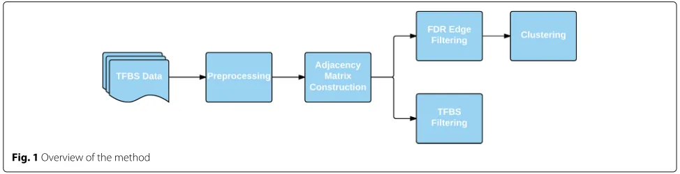
Our method exploited the simple fact that TFs which often interact must have binding sites, as labeled by ChIP-seq or detected by motif searching, near one another, developing a graph with edges weighted by a normal-ized TF-TF co-occurrence score. To calculate this score for each TF-TF pair, we first createdco-occurrence matri-ces, one for each TF, that contained the neighboring TFs at each TFBS of the given transcription factor. These co-occurrence matrices were then transformed to create a series of normalized co-occurrence vectors which con-tained the co-occurrence frequencies for a set of potential TF-TF interactions. These vectors were assembled into the adjacency matrix.
The graph was also used to filter putative TFBSs in order to increase the precision and recall of motif searching, exploiting the fact that motif matches are less likely to be false positives if they fall near the motif matches of their highly co-occurring counterparts. In this case, no FDR fil-tering was done. Instead, summed edge weights were used to threshold and remove putative TFBSs which do not fit the co-occurrence profile in the graph. Figure 1 provides a flowchart overview of our method.
Data sources and preprocessing
We used two datasets in our analysis. The first, the ChIP-seq dataset, used ChIP-seq data for 111 TFs in the cell type K562 from the Encyclopedia of DNA Elements (ENCODE) Project [19]. Each ChIP-seq experiment’s data was uniformly processed by ENCODE to identify the loca-tion of ChIP-seq “peaks”, or ChIP-seq identified TFBSs, within the genome. The TFBSs from the separate exper-iments were assembled and sorted into one large dataset containing over 1.4 million TFBSs. We chose the K562 cell type because it contains the most ChIP-seq data of all cell types within ENCODE. Because TF-TF interactions change between cell types (and in many ways define their different behaviors), the clusters produced by our method were therefore specific to K562.
The second dataset was the ENCODE-motif dataset. To develop ENCODE-motif, Kheradpour and Kellis char-acterized, categorized, and discovered motifs using the ENCODE ChIP-seq experiments, and they provide a col-lection of genomic motif match locations (putative TFBSs) for every motif used in their analysis [20]. This collec-tion contains over 144 million putative TFBSs across 585 transcription factors, and was used in our analysis for clustering of motif-based TFBSs as well as to demonstrate putative TFBS filtering. Kheradpour and Kellis discov-ered motifs as well as characterized known motifs for their analysis; the former were excluded to focus only on pre-established motifs as well as to reduce the size of the dataset somewhat to 124 million putative TFBSs. To reduce its memory requirements, the dataset was divided into 100 segments and one of every four seg-ments was selected, leaving a final total of 31.4 million
putative TFBSs analyzed. If any transcription factor within the ENCODE-motif dataset was represented by multiple motif PWMs, we considered each PWM equivalent, per-forming our clustering and analysis at the TF level rather than the PWM level.
Construction of the adjacency matrix
To construct the adjacency matrix, we first constructed a co-occurrence matrix for each TF in the dataset. To do so, we:
LetTbe the set of all TFs. LetBbe the set of all TFBSs.
LetBtibe TFBSiin the subset ofBencompassing only
the TFBSs of TFt.
Letf(b ∈ B,t ∈ T) = 0 if TF thas no binding sites within 1000 bp of TFBSb, and 1 otherwise.
Then the co-occurrence matrix was ann× mbinary matrix such that
Mt∈T =f(Bt,T)=
⎛ ⎜ ⎝
f(Bt1,T1) . . . f(Btm,T1)
..
. . .. ...
f(Bt1,Tn) . . . f(Btm,Tn)
⎞ ⎟ ⎠
wherenis the length ofTandmis the length ofBt.
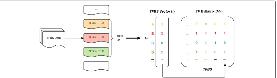
These matrices represent the raw co-occurrence of TFs with one another along the genome; each entry states whether a given TF was found to co-occur (appear within 1000 bp) with another at a particular TFBS. Figure 2 illustrates the construction of these matrices.
Next, a vectorftwas produced for each TFt ∈ Tsuch
that
ft=
⎛ ⎜ ⎝
m
j=1Mt1j
.. . m
j=1Mtnj
⎞ ⎟ ⎠m−1
ft was therefore the row means of Mt for each TF t.
Because Mt is a binary matrix, this produced a vector
of co-occurrence frequencies, where each element rep-resented the fraction of TF t TFBSs where a given TF was found in close proximity. These frequencies, however, were subject to skew due to the overall genomic bind-ing frequencies of their respective TFs. The TF CTCF, for
[image:3.595.55.542.610.735.2]Fig. 2The construction of co-occurrence matrices. For each TFBS of a given TF, the other TFs within a 1000 base-pair window are recorded in that TF’s co-occurrence matrix. The amount of co-occurrence is inversely proportional to the sparsity of the rows; in the above example, TF B is most highly associated with TF D and least associated with TF A
example, binds the genome very frequently, with entire databases devoted to its binding sites, while others, such as GTF2B, bind more rarely [21]. Thus, it is relatively more “important” if GTF2B binds in close proximity to a given TF than CTCF due to CTCF being more prevalent in the background. To account for this, each vectorftwas
normalized such that
ft=ft−fall
with
fall= ⎛ ⎜ ⎝
t∈T
jMt1j
.. .
t∈T
jMtnj
⎞ ⎟ ⎠w−1
whereftis the normalized co-occurrence frequency
vec-tor,wis the length ofB, andfallis theoverallfrequency vector - the row mean of all of theMtmatrices
concate-nated on the horizontal axes.fall was similar to eachft matrix, except while each element in ft represented the co-binding frequencies of a particular TF with TFt, each element infallrepresented the binding frequency of a par-ticular TF to the genome overall. Using the example above, we would expect GTF2B to have a lower entry infallthan CTCF.
Subtracting fall from ft ensured that each element in ftrepresented only the magnitude of the TF-TF
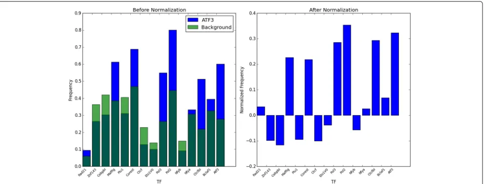
interac-tions, and not the background prevalence of that TF. Using subtraction for normalization penalizes the co-occurrence frequencies evenly; if the subtraction was substituted with division, high-frequency TFs such as CTCF would be overpenalized, while the co-occurrence of low-frequency TFs would be exaggerated. It also allows for negative fre-quencies, a factor which is utilized in the TFBS filtering described later. See Fig. 3 for an example of co-occurrence frequencies before and after normalization.
The adjacency matrixAis constructed by concatenating the normalized co-occurrence frequency vectors such that
A=
⎛ ⎜ ⎝
fT11 . . . fTn1 ..
. . .. ... fT1n . . . fTnn
⎞ ⎟ ⎠
and is used to create an undirected graph where normal-ized co-occurrence frequencies weight edges and TFs are nodes. For the ChIP-seq dataset, the graph contained 111 nodes with 6216 edges. For the ENCODE-motif dataset, the graph contained 585 nodes with 171,405 edges. For the ChIP-seq dataset, construction of the adjacency matrix required 3 min, 52 s on a Core i5-6300U CPU, using less than 5 GB of memory. For the ENCODE-motif dataset, construction of the adjacency matrix required 23 min, 44 s when using four cores in parallel and required less than 14 GB of memory.
Comparing edge weight and motif similarity
An advantage of our method is its ability to detect interac-tions between TFs which are not based on binding motif similarity. That is, if a certain TF binds the genome com-binatorially with other TFs at multiple sequences, a PWM matrix-based clustering method would fail to identify its interactions because of the TF’s weak association with a any particular sequence. Our proximity-based method, however, compares genomic positions rather than PWM matrices, and would therefore be able to detect such interactions.
[image:4.595.58.541.86.222.2]Fig. 3The first fifteen elements in the co-occurrence frequency vector for TF ATF3, shown as a bar graph, before and after normalization. Note how the pre-normalization frequencies of NFYA, ZNF143, and PLU1, which appear significant pre-normalization, are reduced post-normalization
given TF had multiple PWMs. We set up a simple lin-ear regression, examining the extent to which these TF-TF PWM similarity scores predicted our method’s co-occurrence edge weights. We expected a low R2, sig-nifying that motif similarity explained only part of the TF-TF interaction information captured by our method. The results of this analysis are presented in the section “Motif co-occurrence provides more information than similarity alone” in the Results.
Edge filtering using the FPR
Before the graph was clustered, its edges were filtered to remove edges with statistically insignificant weights. While the normalization procedure outlined above did involve subtracting a population mean from a sample mean, this sample was inherently non-random, as the binding sites associated with a TF are non-random. Para-metric methods, then, could not be used to determine an ideal cutoff below which edges can be considered insignif-icant. Instead, an empirical, permuation-based method targeting a user-selected false positive rate (FPR) was employed. In this context, the FPR is the ratio of false posi-tives, or insignificant edges wrongly considered significant (Type I errors), to the total number of truly insignificant edges [22].
In order to determine the edge weight cutoff for a given FPR, the adjacency matrix construction procedure was followed, but the co-occurrence matrices were replaced with dummy matrices. Each row of the dummy matrices was randomly generated, with its sparsity matching that of its overall genomic background frequency (its entry
infall). This created a situation where the overall
preva-lence of TFs was preserved, but their order throughout the genome, and therefore their proximity to other TFs, was randomly shuffled. All edge weights produced in
these circumstances were therefore the result of random fluctuations rather than any real TF-TF associations. For both the ChIP-seq and ENCODE-motif datasets, this pro-cedure was repeated 25 times, generating 308,025 and 8,555,625 dummy edge weights, respectively.
An edge weight threshold was then selected; any edge derived from the dummy matrices with weight greater than this threshold was then a false positive, and any with weight less was a true negative. Thresholds were selected to reach various FPR values, namely 0.01, 0.001, and 0.0001, and these thresholds were used to filter the graph, with any edges with weight lower than the the threshold removed. An FPR of 0.1 was also used for com-parison purposes, to create a baseline graph with many false positive edges against which the three filtered graphs could be compared. This allowed us to assess whether filtering edges using the FPR degraded clustering perfor-mance. Using these FPRs, four new filtered graphs were therefore created for each dataset, which were subse-quently clustered. See Table 1 and the “Results” section for a comparison of clustering at different FPR thresholds.
Comparison to protein-protein interaction data
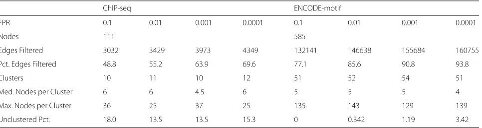
[image:5.595.60.541.86.269.2]Table 1Clustered graph metrics
ChIP-seq ENCODE-motif
FPR 0.1 0.01 0.001 0.0001 0.1 0.01 0.001 0.0001
Nodes 111 585
Edges Filtered 3032 3429 3973 4349 132141 146638 155684 160755
Pct. Edges Filtered 48.8 55.2 63.9 69.6 77.1 85.6 90.8 93.8
Clusters 10 11 10 12 51 52 54 51
Med. Nodes per Cluster 6 6 4.5 6 5 5 5 4
Max. Nodes per Cluster 36 25 37 25 135 143 129 139
Unclustered Pct. 18.0 13.5 13.5 15.3 0 0.342 1.19 3.42
found in the STRING database. The STRING adjacency matrix was then compared with the filtered adjacency matrices produced by our method; a true positive was counted if the two corresponding entries in each matrix were both nonzero. True positives, false positives, true negatives, and false negatives were counted and used to calculate the precision, recall, and F-score of our predicted interactions when compared to the STRING database. For a more in-depth discussion of these metrics, see the section “Filtering of putative TFBSs”. We expected that our predicted interactions would correspond to some extent with the STRING database. However, because our data is TF-specific and derived from TF proximity in reference to the genome rather than the pathways, ontology, and experimental data that underlie STRING interactions, we expected a large number of novel and differing predictions as well.
STRING further splits its interaction scores into seven evidence categories: Co-expression, Experiments, Database, Text-Mining, Neighborhood, Fusion, and Co-occurrence. Given these diverse data sources, we also explored if the interactions detected by our method were significantly more enriched in one of the categories when compared to the others. The Co-expression and Experi-mental categories are the most relevant to our analysis. The Co-expression score describes protein interactions in terms of consistent appearance in expression studies, as would be expected of interacting TFs, and the Exper-iments category describes interactions that have been confirmed in a lab rather than predicted or inferred. The Neighborhood, Fusion, and Co-occurrence evidence channels are least relevant, as they are designed for use in bacteria and archaea protein-protein interaction analy-sis [23]. Therefore, significant enrichment of our method’s STRING matches in the Co-expression and Experimental categories would provide support to our predictions.
MCL clustering
We chose the Markov Clustering Algorithm (MCL), a graph paritioning algorithm, to cluster the filtered net-works. Traditionally, hierarchical clustering, rather than
graph partitioning, has been used for similar tasks, but we believe it bears significant downsides as opposed to a true graph partitioning algorithm such as MCL [24]. First, while hierarchical clustering’s tree output provides an intuitive representation of some inter-cluster relation-ships, “how far up” in the tree to call clusters distinct is not clear. Additionally, hierarchical clustering does not allow nodes to belong to more than one group without dramatically increasing the size of the group. Graph parti-tioning algorithms simply cluster nodes while preserving the structure of the graph, allowing for more relation-ships between nodes and clusters and better exploration. As a result, we chose a partitioning algorithm over a hierarchical clustering algorithm.
In a review by Brohee and van Helden, the MCL algo-rithm was shown to be better suited to clustering protein-protein interactions than three other graph partitioning algorithms, and was therefore chosen for this similar task [25]. We used the MCL algorithm as part of the ClusterMaker suite within graph visualization software Cytoscape for our analysis [26, 27]. The MCL algorithm attempts to partition graphs into clusters by simulat-ing random walks among nodes, where the likelihood of following a given path is based on edge weight. The algorithm then trims paths with the lowest traversal like-lihood and repeats the process. For a full discussion of the algorithm, we refer the reader to Van Dongen’s original publication [28].
MCL depends on three parameters, a granularity parameter, pruning threshold, and an iteration limit; the algorithm’s performance is relatively insensitive to all three. We adjusted only the first, choosing it empirically based on number of clusters produced. Regardless of the dataset or filtering level, the best performing granularity parameter was simple to acquire and always fell between 2 and 5.
Filtering of putative TFBSs
transcription factor ATF3 (the target TF). Here, our method was based on the assumption that a putative TFBS is more likely to be a true positive if it is found near its co-occurring counterparts. We first generated the graph from the ENCODE-motif dataset, but left it unfiltered and did not remove negative edges. Negative edges were helpful in this situation, as the more negative the edge was, theless likely the TF was to be found with the target.
The ChIP-seq dataset was not used for filtering, as its data was the “ground truth.” While the motif PWMs in the ENCODE-motif dataset are derived from ChIP-seq data, the individual putative TFBSs within the ENCODE-motif dataset are found by scanning the PWMs across the genome and checking for matches. As a result, the ENCODE-motif TFBSs are putative, and contain a large number of false positives. In the method below, no infor-mation from the ChIP-seq dataset is used to filter the ENCODE-motif dataset, and therefore, the ChIP-seq data provides a ground truth with which to compare our filter-ing results.
TFBS searching using motifs can be seen as an information-retrieval problem. Information retrieval attempts to maximize the number of relevant “docu-ments” in a pool of retrieved documents [29]. In this case, retrieved documents were the putative TFBSs, and relevant documents were putative TFBSs which matched actual (from ChIP-seq) TFBSs. The performance of information-retrieval systems is often evaluated in terms of recall, precision, and theF-score.
Recall, or sensitivity, is the fraction of relevant doc-uments that are successfully retrieved - the fraction of actual ChIP-seq TFBSs marked by putative motif TFBSs. To determine the recall of the putative TFBSs, a 1000 base-pair window was created around each actual (ChIP-seq determined) ATF3 binding site. The number of actual TFBSs with putative (motif ) TFBSs within their surround-ing window were considered true positives; this sum was divided by the total number of actual TFBSs to produce the recall.
Precision, also known as positive predictive value, is the fraction of retrieved documents that are relevant -the fraction of putative TFBSs that correspond to true ChIP-seq TFBSs. To determine the precision of the puta-tive ATF3 TFBSs, the putaputa-tive TFBSs were first merged, such that any overlapping putative TFBSs were condensed into one larger TFBS. Then the previous procedure was repeated. In this case, however, the 1000 base-pair win-dows were placed around the putative TFBSs and the divisor was the total number of putative ATF3 TFBSs.
TheF-score, the harmonic mean of precision and recall, was also calculated as an overall measure of TFBS search-ing performance.
To maximize precision with a minimal reduction in recall, false putative TFBSs needed to be filtered out
without removing those truly corresponding to ChIP-seq TFBSs. To accomplish this, a “sum-score” was assigned to each putative ATF3 binding site. A 1000 base-pair win-dow was created around each site, and all neighboring TFs within this window were recorded. The score, then, was the sum of all edges from ATF3 to its neighbors within the window. If ATF3 was not often found with a neigh-bor at a given TFBS, the score would be decreased due to a negative edge, and the inverse also held. Thus, if a window contained many highly co-associated TFs, the score was maximized. A threshold was chosen, and all putative TFBSs with scores less than this weight were eliminated. Precision, recall, and theF-score were calcu-lated on the filtered set. To produce a precision recall curve (a close relative of the binary classification reciever operating curve, see [30]) the threshold was adjusted from its minimum (such that no putative TFBSs were removed) to its maximum (such that all TFBSs were removed), and the precision, recall, andF-score were recorded at each point.
We compared the precision-recall curve and maxi-mum F-score from our sum-score with those of three alternate methods. The first removed the same num-ber of TFBSs as the sum-score threshold, but did so randomly, testing if any increase in accuracy was due simply to reduction in the number of TFBSs returned rather than any association between TFs. The second was a score computed simply as the number of neigh-boring TFBSs in each window; it tested if any increase in accuracy was due to the raw number of neighbor-ing TFs (indicatneighbor-ing a possibly highly-active regulatory region). Finally, we calculated a modified sum score, where each window’s score was normalized by the number of TFs within it; this tested whether co-association alone could out-perform the combination of number of neigh-bors and co-association which the unmodified sum-score embodied.
Results
A low FPR yields discrete TF clusters
median nodes per cluster, lower maximum nodes per cluster, and a higher number of clusters.
For the ChIP-seq dataset, FPR 0.01 offered this best bal-ance, while for the ENCODE-motif dataset, FPR 0.001 was the best clustered graph. For both datasets, the median nodes per cluster was manageable, with most nodes congregating in small, interpretable clusters rather than large ones. Between the two datasets, the ratio of clusters to nodes and max nodes per cluster to nodes were similar, but upon visual inspection, the ENCODE-motif dataset appears to perform better, with more clus-ters outside of the large “omnibus” cluster. This is most likely due to the fact that the ENCODE-motif dataset has more nodes to cluster and therefore more clusters to produce. While the images of the entire graph are too large to include in this manuscript with sufficient detail, see the Additional files 1 and 2 section for Cytoscape graph files of the both the ChIP-seq and ENCODE-motif datasets.
When comparing to the high false-positive (FPR=0.1) graphs, we see that good clustering performance was still achieved at low FPRs. We saw that both the ChIP-seq and ENCODE-motif datasets performed equally to the base-line high-FPR (0.1) in terms of clusters, median nodes per cluster, and maximum nodes per cluster, but differed in terms of unclustered percentage. For the ENCODE-motif dataset, we observed the intuitive increase in unclustered nodes as the FPR, and therefore the number of edges fil-tered, increased. As FPR increased and more edges were cut, more nodes would become disconnected and there-fore unclustered.
The ChIP-seq dataset, however, showed the opposite trend, with the high-FPR (less edges filtered) dataset having more unclustered nodes. This is due to the low percentage of edges filtered at this FPR. The 0.1 FPR ChIP-seq graph filters only 48.8% of the edges, while the ENCODE-motif graph still filters 77.1%. We observed that the MCL algorithm failed to adequately cluster the data when there were too many edges included, leaving larger “omnibus” clusters and more unclustered nodes. The FPR of 0.1 for the ChIP-seq dataset, then, failed to trim enough edges, causing an increase in the number of unclustered nodes.
In this way, FPR acts as a tuning parameter. Increas-ing it reduces noise at the cost of disconnectIncreas-ing nodes and increasing unclustered nodes. Decreasing it increases noise while allowing more nodes to be clustered, up to the point that too few edges are filtered and MCL fails to adequately cluster the nodes.
TF clusters agree with known TF-TF interactions
Many of the ChIP-seq and ENCODE-motif datasets’ clus-ters embodied known TF-TF interactions, lending cre-dence to our method’s accuracy. The ChIP-seq FPR 0.001
graph includes the experimentally known SM3A-CTCF, JUN-FOS, TAL1-EGR1, JUN-NFY, STAT1-GATA1, and ELK1-STAT2 interactions, among others [31–36] .
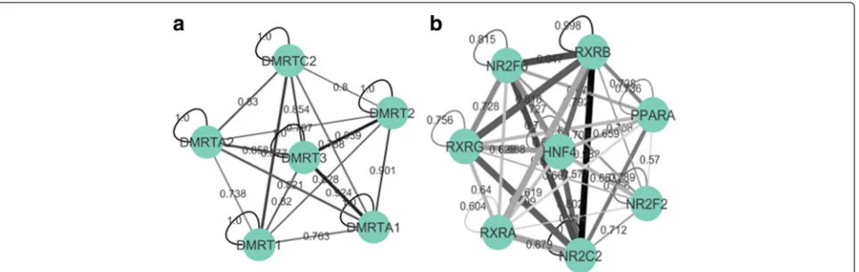
Many clusters from the ENCODE-motif dataset group the different motifs from the same family, such as the DMRT family in Fig. 6. This is expected, as motif PWMs within the same family would be expected to be highly similar. Other clusters, however, include both intra- and extra-familial interactions, and these contain the known CREB-ATF, BACH-NFE2, NFIL3-HLF, NR2F-HNF (see Fig. 6), and YY-SRF interactions, among others [37–41].
When compared to the STRING protein-protein inter-action database, the ChIP-seq dataset has a recall of 0.4342, a precision of 0.3736, and an F-Score of 0.4016, with the FPR=0.01 graph performing best. The ENCODE-motif dataset has a recall of 0.2051, a precision of 0.2282, and an F-Score of 0.2161, with the FPR=0.01 graph again performing best. Because our method finds TF-TF interactions based on genomic colocation and is entirely focused on transcription factors, while STRING is focused on all protein-protein interactions and derives its interac-tions from very diverse data sources, it is expected that our method would produce many novel predictions when compared to STRING. Even so, 37% (over 4000) and 22% (over 75,000) of the TF-TF interactions predicted by our method were also contained within the STRING database for the ChIP-seq and ENCODE-motif datasets, respec-tively, and our precision and recall values correspond to those of several otherin silicoprotein-protein interaction prediction methods [11, 42–47]
For the ChIP-seq and ENCODE-motif datasets, we found that our method identified TF-TF interactions which were significantly (p < 0.05 and p < 0.001, respectively) more enriched in the Co-expression evi-dence category when compared to STRING interactions which were not predicted by our method. This indicates that our method preferentially identifies interactions con-taining TFs that are consistently present in the same cell at the same time, as would be expected of interacting TFs. The ENCODE-motif dataset is also significantly enriched in the Experimental, Database, and Text-mining cate-gories (p<0.001 for each). The Experiment and Database enrichment is especially important, as it provides evi-dence that our method preferentially captures interactions which have been experimentally derived. Figure 4 com-pares the evidence category enrichments for out method’s TF-TF interactions.
Fig. 4A comparison of STRING evidence category enrichments between STRING interactions which matched our predicted TF-TF interactions and those that did not, for (a) the ChIP-seq dataset, and (b) the ENCODE-motif dataset
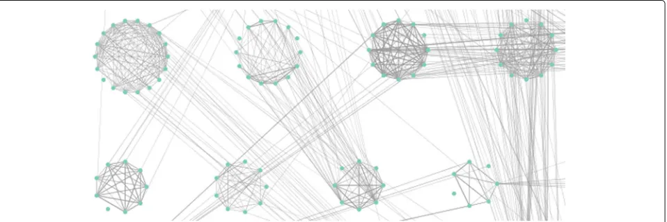
interactions on a putative basis. Also, unlike experimen-tal assays which are blind to the larger framework the complexes they detect may participate in, our method preserves cluster edges, leaving cluster-cluster inter-actions (see Fig. 5) or single-TF many-cluster interac-tions free to be explored. Additionally, while the clusters assigned by our method are putative, we believe the accu-racy, cheapness, and speed of our method allows it to be used as a springboard by which to direct future research, allowing experimental investigators to start with potential TF-TF interactions instead of “from scratch.”
Motif co-occurrence provides more information than similarity alone
A potential advantage of our method is its ability to detect TF interactions outside the realm of motif PWM similar-ity. The regression outlined in “Comparing edge weight and motif similarity” showedR2to be 0.262, indicating
that motif similarity accounted for only 26.2% of the variance in normalized edge weight. This implies that motif similarity does not automatically equal motif co-occurrence, especially when co-occurrence is normalized against total background occurrence as it has been in our method.
Practically, this can mean the difference between spot-ting a TF-TF interaction and missing one. In Fig. 6, our method grouped the TFs together regardless of the fact that their PWM similarities (signified by edge darkness) are largely inconsistent, with some interactions within the cluster having highly similar motifs and others weak motif similarity. A similarity-based method would fail to group the experimentally validated HNF-NR2F2 interac-tion found in this cluster due their PWM dissimilarity (lighter gray edge in Fig. 6), but our method was able cap-ture the interaction because they co-occur often (thicker edge in Fig. 6).
[image:9.595.58.541.86.233.2] [image:9.595.62.541.544.704.2]Fig. 6Two clusters from the ENCODE-motif dataset, with edge thickness representing the co-occurrence frequency edge weight generated by our method, and edge color (light gray to dark black) representing PWM similarity (used in similarity-based methods). In (a), all of the TFs are from the same family (DMRT), and therefore have high levels of motif similarity (all the edges are dark). Our method is able to group them together because they co-occur often. In (b), the grouping has both intra- and extra-familial connections, with some TFs having dissimilar (light gray) PWMs. Many of these interactions could not be picked up a motif similarity-based method
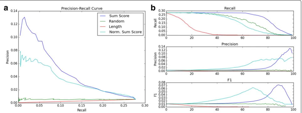
Filtering of putative TFBSs significantly improves accuracy Without filtering, the recall of ATF3’s putative TFBSs was 0.277, while the precision was only 0.0053, giving anF-score of 0.0104. Our method achieved a maximum F-score of 0.0725, an increase of nearly seven times the unfiltered F-score, and increased precision by a factor 12.6 to 0.0667. At the same time, recall at the maximum F-score only decreased by a factor of 3.4 to 0.0795. Addi-tionally, if the recall is held at the original, unfiltered level of 0.277, the normalized sum-score doubles the unfil-tered precision, at 0.0104. It should be noted that this was achieved in a completely unsupervised manner, with ground truth experimental ChIP-seq data used only to determine after-the-fact accuracy.
Several interesting observations were taken from Fig. 7. We found that the non-normalized sum score performed the best compared to the other scores evaluated, achieving the slowest drop in recall, the greatest increase in preci-sion, and the best overall precision-recall curve. Both the non-normalized and normalized sum-scores performed much better than the random-removal null metric, indi-cating that the motif co-occurrence used to create our score truly captures information that allows it separate true putative TFBSs from false ones.
Additionally, the number of TFs in each TFBS win-dow performed significantlyworsethan both the random removal and sum-score, with no increase in precision and a faster decrease in recall. Upon further investiga-tion, we found that number of neighboring TFBSs was actually stronglynegativelycorrelated with the sum-score (R = −0.81). We flipped the thresholding to account for this, such that the cutoffs went from high num-ber of neighbors to low (reflected in the corresponding curve in Fig. 7), but the performance was still worse than random. This meant that “quality” of neighboring TFs
was more important than “quantitity” when filtering; as the number of neighboring TFs increased, more erro-neous TFs with negative edge weights crept in, decreasing the score.
At the same time, however, the non-normalized sum-score performed marginally better than the normalized sum-score, meaning that removing the effect of the num-ber of neighboring TFs in each window altogether was detrimental rather than helpful. We believe this is due to a “boosting” effect which the non-normalized sum-score allows. In a situation where a putative TFBS not only has frequently co-occurring neighbors but the added benefit ofmanyof them, the non-normalized score takes this into account while the normalized cannot, giving the non-normalized score a slight performance advantage.
While the normalized sum-score performed slightly worse in terms of raw F-score, it cannot be discounted, as the normalized score achieved only slightly lower metrics while maintaining a lower cutoff value. This meant that the normalized score left more TFBSs in the filtered set, which would be ideal if further processing on the filtered set was desired.
[image:10.595.59.541.86.239.2]Fig. 7 aThe precision-recall curve for TFBS filtering of ATF3. A more gradual decrease in precision with the increase in recall signifies better performance. “Length” indicates the score based on the number of neighboring TFBSs within each window.bThe recall, precision, andF-score plotted as the cutoff (number of filtered TFBSs) increases
Discussion
The TF regulatory framework is essential to cellular regulation and human health but is difficult to under-stand, with interactions between TFs and the genome as well as between TFs themselves. While established methods exist to locate where TFs bind the genome, the clustering and interaction of TFs themselves is largely unexplored. Many clustering methods use motif PWM similarity, which leaves out interactions not based on sequence affinity, and methods which use proximity data from ChIP-seq or motif analysis have not been applied to true TF clustering. In this study, we presented a proximity-based graph clustering solution for the identification of TF clusters.
We used TF co-occurrence data from two TFBS datasets to develop graphs, which were then filtered using an empirical FPR thresholding method. MCL was applied to the filtered graphs, producing many distinct, manage-able clusters, with the motif-based dataset performing best. Good clustering performance was achieved even at very low FPRs where as much as 94% of graph edges were filtered out. FPR represented a trade-off parameter; a decreased FPR would decrease the maximum nodes per cluster and increased the total number of clusters, but this increased the number of orphaned, unclustered TFs.
Furthermore, we believe that our results provide evi-dence that clusters produced by our method are accurate and correspond to biological realities. First, many experi-mentally known TF-TF interactions were identified within our graphs’ clusters, and our graphs correspond well to the protein-protein interactions found in the STRING database, indicating on an empirical basis that our high-throughput, one-pass method is capable of accurate clus-ter assignment. Our use of the MCL algorithm leaves
inter-cluster edges intact, which more closely mirrors the biological reality of a highly-connected, complex regula-tory system and allows for further exploration of TF-TF and cluster-cluster interactions.
Second, the information contained within the graph structure was able to significantly improve the accuracy of motif-based TFBS searching for the TF ATF3 when compared to ground truth ChIP-seq data, which indi-cates that the co-occurrence of TFs with one another has direct biological relevance. Our filtering was based on the simple assumption that if a given TF tends to co-occur with a set of other TFs, a putative binding site without the frequently co-occurring TFs is likely to be a false positive. The unfiltered, unclustered graph was used to generate scores for each putative TFBS, and TFBSs with scores below a certain threshold were filtered out. The precision-recall curves for the graph-based scores significantly outperformed those graph-based on number (rather than identity) of co-occurring TFs as well as a random control. The TF-TF relationships iden-tified by our method must therefore have a biologi-cal basis, as they bring the accuracy of motif-based TFBS searching closer to that of the ChIP-seq biological reality.
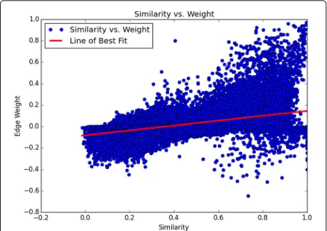
Finally, by regressing motif PWM similarity with the edges of our graph, we demonstrated that our method captures information beyond PWM similarity in the ENCODE-motif dataset. PWM similarity only accounted for 25% of the variance within our TF-TF associations, allowing for TF-TF interactions to be found where they otherwise would be missed (Fig. 8).
Fig. 8Motif similarity poorly predicts the edge weight used in our analysis, indicating that our method can capture interactions that extend beyond motif similarity
it does so on a putative basis, and it does not offer a quan-titative level of likelihood for the clusters it produces. Our method, however, is not meant to replace experimental investigation or confirmation of TF clusters. Instead, it is meant as a tool to quickly and easily explore TF-TF inter-actions on a putative basis. Additionally, when used with ChIP-seq datasets taken from different cell types or under different cellular conditions, it allows for direct visual-ization of how TF clusters, and therefore the regulatory environment, change from cell to cell and condition to condition.
Conclusions
Transcription factors form a complex regulatory network which is crucial to human health but is difficult to under-stand. Methods such as ChIP-seq and motif searching can identify where a TF is likely to bind, but TFs also interact among themselves in ways that are largely unex-plored. To address this, we used TF co-occurrence data to develop filtered, normalized graphs, with edges represent-ing the degree of association between TFs. We clustered these graphs using the MCL algorithm, which produced many distinct clusters with known TF-TF interactions while preserving inter-cluster edges. We also demon-strated that our proximity-based co-occurrence method captures information, and therefore TF interactions, that PWM similarity methods cannot. The biological corre-spondence of our graph output was also demonstrated when we compared it to protein-protein interactions in the STRING database, as well as when we used the graph structure to filter putative TFBSs for ATF3, significantly reducing the number of false positives and increasing accuracy. Going forward, this method can be applied to
examine how TF clusters change between cellular con-ditions and cell types, opening doors into the “second dimension” of TF regulatory dynamics.
Additional files
Additional file 1: chip_graphs.cys.Cytoscape file of the ChIP-seq dataset graph and its clustered graphs as described in the Results section. (CYS 318 kb)
Additional file 2: motif_graphs.cys.Cytoscape file of the ENCODE-motif dataset graph and its clustered graphs as described in the Results section. (CYS 9216 kb)
Acknowledgements
MS wishes to thank Dr. Kerby Shedden of the University of Michigan Department of Statistics for his assistance and advice regarding the work.
Funding
Project supported by NSF CAREER Award DBI-1651614 (APB).
Availability of data and materials
The ChIP-seq dataset is available from the ENCODE project, at http://genome. ucsc.edu/ENCODE/dataMatrix/encodeChipMatrixHuman.html [19]. The ENCODE-motif dataset is available at http://compbio.mit.edu/encode-motifs/ [20].
The Cytoscape graph files supporting the results of this article are included with the article (and its Additional files 1 and 2).
Authors’ contributions
MS developed the method, analyzed the data, and wrote the manuscript. KN and AB provided substantial feedback on method conceptualization and implementation, as well as revisions for the manuscript. All authors read and approved the final manuscript.
Ethics approval and consent to participate Not applicable.
Consent for publication Not applicable.
Competing interests
The authors declare that they have no competing interests.
Publisher’s Note
Springer Nature remains neutral with regard to jurisdictional claims in published maps and institutional affiliations.
Author details
1University of Michigan Medical School, 1301 Catherine, 48109-5624 Ann
Arbor, USA.2University of Michigan Department of Computational Medicine and Bioinformatics, 100 Washtenaw Avenue, 48109 Ann Arbor, USA. 3University of Michigan Medical School Department of Emergency Medicine,
1500 E Medical Center Drive, 48109 Ann Arbor, USA.4University of Michigan Department of Genetics, 1241 E Catherine, 48109 Ann Arbor, USA.
Received: 26 June 2017 Accepted: 14 November 2017
References
1. Vaquerizas JM, Kummerfeld SK, Teichmann SA, Luscombe NM. A census of human transcription factors: function, expression and evolution. Nat Rev Genet. 2009;10(4):252–63. doi:10.1038/nrg2538. Accessed 21 Jan 2016.
[image:12.595.56.291.87.253.2]3. Accili D, Arden KC. FoxOs at the Crossroads of Cellular Metabolism, Differentiation, and Transformation. Cell. 2004;117(4):421–6. doi:10.1016/S0092- 8674(04)00452-0. Accessed 21 Jan 2016.
4. Bain G, Maandag ECR, Izon DJ, Amsen D, Kruisbeek AM, Weintraub BC, Krop I, Schlissel MS, Feeney AJ, van Roon M, van der Valk M, te Riele HPJ, Berns A, Murre C. E2A proteins are required for proper B cell development and initiation of immunoglobulin gene rearrangements. Cell. 1994;79(5): 885–92. doi:10.1016/0092-8674(94)90077-9. Accessed 21 Jan 2016. 5. Boyadjiev S, Jabs E. Online Mendelian Inheritance in Man (OMIM) as a
knowledgebase for human developmental disorders. Clin Genetics. 2000;57(4):253–66. doi:10.1034/j.1399-0004.2000.570403.x. Accessed 2016-01-21.
6. Collas P. The Current State of Chromatin Immunoprecipitation. Mol Biotechnol. 2010;45(1):87–100. doi:10.1007/s12033-009-9239-8. Accessed 05 Apr 2016.
7. Park PJ. ChIP–seq: advantages and challenges of a maturing technology. Nat Rev Genetics. 2001;10(10):669–80. doi:10.1038/nrg2641. Accessed 26 Jan 2016.
8. Kel AE, Gößling E, Reuter I, Cheremushkin E, Kel-Margoulis OV, Wingender E. MATCHTM: a tool for searching transcription factor binding sites in DNA sequences. 31(13):3576–9. doi:10.1093/nar/gkg585. 12824369 Accessed 05 Apr 2016.
9. Beckstette M, Homann R, Giegerich R, Kurtz S. Fast index based algorithms and software for matching position specific scoring matrices. BMC Bioinformatics. 2006;389(7). doi:10.1186/1471-2105-7-389. Accessed 05 Apr 2016.
10. Burley SK, Kamada K. Transcription factor complexes. Curr Opin Struct Biol. 2002;12(2):225–30. doi:10.1016/S0959-440X(02)00314-7. Accessed 21 Jan 2016.
11. Xie D, Boyle AP, Wu L, Zhai J, Kawli T, Snyder M. Dynamic trans-Acting Factor Colocalization in Human Cells. Cell. 2013;155(3):713–24. doi:10.1016/j.cell.2013.09.043.
12. Roder K, Wolf SS, Larkin KJ, Schweizer M. Interaction between the two ubiquitously expressed transcription factors NF-Y and Sp1. 234(1):61–9. 10393239.
13. Tshori S, Nechushtan H. Mast cell transcription factors—Regulators of cell fate and phenotype. Biochim Biophys Acta (BBA) - Mol Basis Dis. 2012;1822(1):42–8. doi:10.1016/j.bbadis.2010.12.024. Accessed 26 Jan 2016.
14. Igarashi K, Kataoka K, Itoh K, Hayashi N, Nishizawa M, Yamamoto M. Regulation of transcription by dimerization of erythroid factor NF-E2 p45 with small Maf proteins. 367(6463):568–72. doi:10.1038/367568a0.8107826. 15. Grau J, Grosse I, Posch S, Keilwagen J. Motif clustering with implications for transcription factor interactions. PeerJ. 2015. doi:10.7287/peerj.preprints. 1302v1. Accessed Apr 2016.
16. Xu M, Su Z. A Novel Alignment-Free Method for Comparing Transcription Factor Binding Site Motifs. PLOS ONE. 2010;5(1):8797.
doi:10.1371/journal.pone.0008797. Accessed 05 Apr 2016.
17. Frith MC, Li MC, Weng Z. Cluster-Buster: finding dense clusters of motifs in DNA sequences. 31(13):3666–8. doi:10.1093/nar/gkg540.12824389. Accessed 05 Apr 2016.
18. Murakami K, Kojima T, Sakaki Y. Assessment of clusters of transcription factor binding sites in relationship to human promoter, CpG islands and gene expression. BMC Genomics. 2004;5(16). doi:10.1186/1471-2164-5-16. Accessed 05 Apr 2016.
19. Consortium TEP. An integrated encyclopedia of DNA elements in the human genome. Nature. 2012;7414(489):57–74. doi:10.1038/nature11247. Accessed 26 Jan 2016.
20. Kheradpour P, Kellis M. Systematic discovery and characterization of regulatory motifs in ENCODE TF binding experiments. Nucleic Acids Res. 2014;42(5):2976–87. doi:10.1093/nar/gkt1249. Accessed 07 Apr 2016. 21. Ziebarth JD, Bhattacharya A, Cui Y. CTCFBSDB 2.0: a database for
CTCF-binding sites and genome organization. 41:188–94. doi:10.1093/nar/gks1165.23193294. Accessed 07 Apr 2016. 22. Shaffer JP. Multiple Hypothesis Testing. Annu Rev Psychol. 1995;46(1):
561–84. doi:10.1146/annurev.ps.46.020195.003021. Accessed 07 Apr 2016. 23. Szklarczyk D, Franceschini A, Wyder S, Forslund K, Heller D, Huerta-Cepas J, Simonovic M, Roth A, Santos A, Tsafou KP, Kuhn M, Bork P, Jensen LJ, von Mering C. STRING v10: protein–protein interaction networks, integrated over the tree of life. Nucleic Acids Res. 2015;43:447–52. doi:10.1093/nar/gku1003.
24. Wang J, Li M, Deng Y, Pan Y. Recent advances in clustering methods for protein interaction networks. 11(10). doi:10.1186/1471-2164-11-S3-S10. 21143777. Accessed 08 Apr 2016.
25. Brohée S, van Helden J. Evaluation of clustering algorithms for protein-protein interaction networks. BMC Bioinformatics. 2006;7:488. doi:10.1186/1471-2105-7-488. Accessed 26 Jan 2016.
26. Morris JH, Apeltsin L, Newman AM, Baumbach J, Wittkop T, Su G, Bader GD, Ferrin TE. clusterMaker: a multi-algorithm clustering plugin for Cytoscape. BMC Bioinformatics. 2011;12:436. doi:10.1186/1471-2105-12-436. Accessed 07 Apr 2016.
27. Shannon P, Markiel A, Ozier O, Baliga NS, Wang JT, Ramage D, Amin N, Schwikowski B, Ideker T. Cytoscape: a software environment for integrated models of biomolecular interaction networks. 13(11): 2498–504. doi:10.1101/gr.1239303.14597658.
28. Van Dongen S. A Cluster algorithm for graphs. Inf Syst. 2000;10:1–40. Accessed 26 Jan 2016.
29. Singhal A. Modern information retrieval: a brief overview. Mod Inf Retrieval. 2001;24(4):35–43.
30. Davis J, Goadrich M. The Relationship Between Precision-Recall and ROC Curves. In: Proceedings of the 23rd International Conference on Machine Learning. ICML ’06. ACM. p. 233–240. doi:10.1145/1143844.1143874. http://doi.acm.org/10.1145/1143844.1143874. Accessed 10 Apr 2016. 31. Degner SC, Verma-Gaur J, Wong TP, Bossen C, Iverson GM, Torkamani A,
Vettermann C, Lin YC, Ju Z, Schulz D, Murre CS, Birshtein BK, Schork NJ, Schlissel MS, Riblet R, Murre C, Feeney AJ. CCCTC-binding factor (CTCF) and cohesin influence the genomic architecture of the Igh locus and antisense transcription in pro-B cells. 108(23):9566–71. doi:10.1073/pnas. 1019391108.21606361. Accessed 26 Jan 2016.
32. Chiu R, Boyle WJ, Meek J, Smeal T, Hunter T, Karin M. The c-Fos protein interacts with c-Jun/AP-1 to stimulate transcription of AP-1 responsive genes. 54(4):541–52. 3135940.
33. Tang T, Arbiser JL, Brandt SJ. Phosphorylation by Mitogen-activated Protein Kinase Mediates the Hypoxia-induced Turnover of the TAL1/SCL Transcription Factor in Endothelial Cells. 277(21):18365–72. doi:10.1074/ jbc.M109812200.11904294. Accessed 12 Apr 2016.
34. Su M, Bansal AK, Mantovani R, Sodek J. Recruitment of Nuclear Factor Y to the Inverted CCAAT Element (ICE) by c-Jun and E1A Stimulates Basal Transcription of the Bone Sialoprotein Gene in Osteosarcoma Cells. 280(46):38365–75. doi:10.1074/jbc.M501609200.16087680. Accessed 12 Apr 2016.
35. Klampfer L, Huang J, Corner G, Mariadason J, Arango D, Sasazuki T, Shirasawa S, Augenlicht L. Oncogenic Ki-Ras Inhibits the Expression of Interferon-responsive Genes through Inhibition of STAT1 and STAT2 Expression. 278(47):46278–87. doi:10.1074/jbc.M304721200.12972432. Accessed 12 Apr 2016.
36. Huang Z, Richmond TD, Muntean AG, Barber DL, Weiss MJ, Crispino JD. STAT1 promotes megakaryopoiesis downstream of GATA-1 in mice. 117(12):3890–9. doi:10.1172/JCI33010.18060035. Accessed 13 Apr 2016. 37. Hummler E, Cole TJ, Blendy JA, Ganss R, Aguzzi A, Schmid W,
Beermann F, Schütz G. Targeted mutation of the CREB gene: compensation within the CREB/ATF family of transcription factors. 91(12):5647–51. 8202542. Accessed 12 Apr 2016.
38. Oyake T, Itoh K, Motohashi H, Hayashi N, Hoshino H, Nishizawa M, Yamamoto M, Igarashi K. Bach proteins belong to a novel family of BTB-basic leucine zipper transcription factors that interact with MafK and regulate transcription through the NF-E2 site. 16(11):6083–95. 8887638. Accessed 13 Apr 2016.
39. Ikushima S, Inukai T, Inaba T, Nimer SD, Cleveland JL, Look AT. Pivotal role for the NFIL3/E4BP4 transcription factor in interleukin 3-mediated survival of pro-B lymphocytes. 94(6):2609–14. 9122243. Accessed 13 Apr 2016.
40. Beaudet MJ, Desrochers M, Lachaud AA, Anderson A. The CYP2B2 phenobarbital response unit contains binding sites for hepatocyte nuclear factor 4, PBX-PREP1, the thyroid hormone receptor beta and the liver X receptor. 388:407–18. doi:10.1042/BJ20041556.15656786. Accessed 13 Apr 2016.
41. Gualberto A, LePage D, Pons G, Mader SL, Park K, Atchison ML, Walsh K. Functional antagonism between YY1 and the serum response
factor. 12(9):4209–14. 1508214. Accessed 13 Apr 2016.
template-based and de novo docking methods. BMC Proceedings. 2013;7(6). doi:10.1186/1753-6561-7-S7-S6.
43. Ohue M, Matsuzaki Y, Uchikoga N, Ishida T, Akiyama Y. MEGADOCK: an all-to-all protein-protein interaction prediction system using tertiary structure data. Protein Pept Lett. 2014;21(8):766–78.
44. Kolchinsky A, Abi-Haidar A, Kaur J, Hamed AA, Rocha LM. Classification of protein-protein interaction full-text documents using text and citation network features. IEEE Xplore. 2010;7(3):400–11.
doi:10.1109/TCBB.2010.55.
45. Rual JF, Venkatesan K, Hao T, Hirozane-Kishikawa T, Dricot A, Li N, Berriz GF, Gibbons FD, Dreze M, Ayivi-Guedehoussou N, Klitgord N, Simon C, Boxem M, Milstein S, Rosenberg J, Goldberg DS, Zhang LV, Wong SL, Franklin G, Li S, Albala JS, Lim J, Fraughton C, Llamosas E, Cevik S, Bex C, Lamesch P, Sikorski RS, Vandenhaute J, Zoghbi HY, Smolyar A, Bosak S, Sequerra R, Doucette-Stamm L, Cusick ME, Hill DE, Roth FP, Vidal M. Towards a proteome-scale map of the human protein–protein interaction network. Nature. 2005;437(7062):1173–8. doi:10.1038/nature04209. Accessed 28 Oct 2017.
46. Keskin O, Nussinov R, Gursoy A. PRISM: protein-protein interaction prediction by structural matching. Methods Mol Biol. 2008;484:505–21. 47. Zeng E, Ding C, Narasimhan G, Holbrook SR. Estimating support for
protein-protein interaction data with applications to function prediction. Comput Syst Bioinformatics Conf. 2008;7:73–84.
• We accept pre-submission inquiries
• Our selector tool helps you to find the most relevant journal
• We provide round the clock customer support
• Convenient online submission
• Thorough peer review
• Inclusion in PubMed and all major indexing services
• Maximum visibility for your research
Submit your manuscript at www.biomedcentral.com/submit