New construction and proof techniques of projection algorithm for countable maximal monotone mappings and weakly relatively non expansive mappings in a Banach space

R E S E A R C H

Open Access

New construction and proof techniques of

projection algorithm for countable maximal

monotone mappings and weakly relatively

non-expansive mappings in a Banach space

Li Wei

_{and Ravi P. Agarwal}

*_{Correspondence:}

[email protected]

1_{School of Mathematics and}

Statistics, Hebei University of Economics and Business, Shijiazhuang, China

Full list of author information is available at the end of the article

Abstract

In a real uniformly convex and uniformly smooth Banach space, some new monotone projection iterative algorithms for countable maximal monotone mappings and countable weakly relatively non-expansive mappings are presented. Under mild assumptions, some strong convergence theorems are obtained. Compared to corresponding previous work, a new projection set involves projection instead of generalized projection, which needs calculating a Lyapunov functional. This may reduce the computational labor theoretically. Meanwhile, a new technique for finding the limit of the iterative sequence is employed by examining the relationship

between the monotone projection sets and their projections. To check the

effectiveness of the new iterative algorithms, a specific iterative formula for a special example is proved and its computational experiment is conducted by codes of Visual Basic Six. Finally, the application of the new algorithms to a minimization problem is exemplified.

MSC: 47H05; 47H09; 47H10

Keywords: Maximal monotone mapping; Weakly relatively non-expansive mapping; Projection; Limit of a sequence of sets; Uniformly convex and uniformly smooth Banach space

1 Introduction and preliminaries

LetEbe a real Banach space withE∗its dual space. Suppose thatCis a nonempty closed and convex subset ofE. The symbol·,·denotes the generalized duality pairing between

EandE∗. The symbols “→” and “” denote strong and weak convergence either inEor inE∗, respectively.

A Banach spaceEis said to be strictly convex [1] if for∀x,y∈Ewhich are linearly inde-pendent,

x+y<x+y.

The above inequality is equivalent to the following:

x=y= 1, x=y ⇒ x+y

2

< 1.

A Banach spaceEis said to be uniformly convex [1] if for any two sequences{xn}and {yn}inEsuch thatxn=yn= 1 andlimn→∞xn+yn= 2,limn→∞xn–yn= 0 holds.

IfEis uniformly convex, then it is strictly convex.

The functionρE: [0, +∞)→[0, +∞) is called the modulus of smoothness ofE[2] if it is defined as follows:

ρE(t) =sup

1 2

x+y+x–y– 1 :x,y∈E,x= 1,y ≤t

.

A Banach spaceEis said to be uniformly smooth [2] if ρE(t)

t →0, ast→0. The Banach spaceEis uniformly smooth if and only ifE∗is uniformly convex [2]. We sayE has Property (H) if for every sequence{xn} ⊂Ewhich converges weakly to

x∈Eand satisfiesxn → xasn→ ∞necessarily converges toxin the norm. IfEis uniformly convex and uniformly smooth, thenEhas Property (H). With eachx∈E, we associate the set

J(x) =f ∈E∗:x,f=x2=f2, ∀x∈E.

Then the multi-valued mappingJ:E→2E∗_{is called the normalized duality mapping} [1]. Now, we list some elementary properties ofJ.

Lemma 1.1([1, 2])

(1) IfEis a real reflexive and smooth Banach space,thenJis single valued;

(2) ifEis reflexive,thenJis surjective;

(3) ifEis uniformly smooth and uniformly convex,thenJ–1_{is also the normalized} duality mapping fromE∗intoE.Moreover,bothJandJ–1_{are uniformly continuous} on each bounded subset ofEorE∗,respectively;

(4) forx∈Eandk∈(–∞, +∞),J(kx) =kJ(x).

For a nonlinear mappingU, we useF(U) andN(U) to denote its fixed point set and null point set, respectively; that is,F(U) ={x∈D(U) :Ux=x}andN(U) ={x∈D(U) :Ux= 0}.

Definition 1.2([3]) A mappingT⊂E×E∗is said to be monotone if, for∀yi∈Txi,i= 1, 2, we havex1–x2,y1–y2 ≥0. The monotone mappingT is called maximal monotone if

R(J+θT) =E∗forθ> 0.

Definition 1.3([4]) The Lyapunov functional ϕ:E×E∗ →(0, +∞) is defined as

fol-lows:

Definition 1.4([5]) LetB:C→Cbe a mapping, then

(1) an elementp∈Cis said to be an asymptotic fixed point ofBif there exists a sequence{xn}inCwhich converges weakly topsuch thatxn–Bxn→0, asn→ ∞. The set of asymptotic fixed points ofBis denoted byFˆ(B);

(2) B:C→Cis said to be strongly relatively non-expansive ifFˆ(B) =F(B) =∅and ϕ(p,Bx)≤ϕ(p,x)forx∈Candp∈F(B);

(3) an elementp∈Cis said to be a strong asymptotic fixed point ofBif there exists a sequence{xn}inCwhich converges strongly to p such thatxn–Bxn→0, as

n→ ∞. The set of strong asymptotic fixed points ofBis denoted byF˜(B); (4) B:C→Cis said to be weakly relatively non-expansive ifF˜(B) =F(B) =∅and

ϕ(p,Bx)≤ϕ(p,x)forx∈Candp∈F(B).

Remark1.5 It is easy to see that strongly relatively non-expansive mappings are weakly relatively non-expansive mappings. However, an example in [6] shows that a weakly rela-tively non-expansive mapping is not a strongly relarela-tively non-expansive mapping.

Lemma 1.6([5]) Let E be a uniformly convex and uniformly smooth Banach space and C be a nonempty closed and convex subset of E.If B:C→C is weakly relatively non-expansive,then F(B)is a closed and convex subset of E.

Lemma 1.7([3]) Let T⊂E×E∗be maximal monotone,then

(1) N(T)is a closed and convex subset ofE;

(2) ifxn→xandyn∈Txnwithyny,orxnxandyn∈Txnwithyn→y,then

x∈D(T)andy∈Tx.

Definition 1.8([4])

(1) IfEis a reflexive and strictly convex Banach space andCis a nonempty closed and convex subset ofE, then for eachx∈Ethere exists a unique elementv∈Csuch thatx–v=inf{x–y:y∈C}. Such an elementvis denoted byPCxandPCis called the metric projection ofEontoC.

(2) LetEbe a real reflexive, strictly convex, and smooth Banach space andCbe a nonempty closed and convex subset ofE, then for∀x∈E, there exists a unique elementx0∈Csatisfyingϕ(x0,x) =inf{ϕ(y,x) :y∈C}. In this case,∀x∈E, define C:E→CbyCx=x0, and thenCis called the generalized projection fromE ontoC.

It is easy to see thatCis coincident withPCin a Hilbert space.

In [12], Wei et al. presented the following iterative algorithms to approximate a common element of the set of null points of the maximal monotone mappingT⊂E×E∗and the set of fixed points of the strongly relatively non-expansive mappingS⊂E×E, whereEis a real uniformly convex and uniformly smooth Banach space:

⎧ ⎪ ⎪ ⎪ ⎪ ⎪ ⎪ ⎪ ⎪ ⎪ ⎪ ⎪ ⎪ ⎪ ⎪ ⎪ ⎪ ⎪ ⎨ ⎪ ⎪ ⎪ ⎪ ⎪ ⎪ ⎪ ⎪ ⎪ ⎪ ⎪ ⎪ ⎪ ⎪ ⎪ ⎪ ⎪ ⎩

x1∈E, r1> 0,

yn= (J+rnT)–1J(xn+en),

zn=J–1[αnJxn+ (1 –αn)Jyn],

un=J–1[βnJxn+ (1 –βn)JSzn],

Hn={z∈E:ϕ(z,zn)≤αnϕ(z,xn) + (1 –αn)ϕ(z,xn+en)},

Vn={z∈E:ϕ(z,un)≤βnϕ(z,xn) + (1 –βn)ϕ(z,zn)},

Wn={z∈E:z–xn,Jx1–Jxn ≤0},

xn+1=Hn∩Vn∩Wn(x1), n∈N,

(1.1) ⎧ ⎪ ⎪ ⎪ ⎪ ⎪ ⎪ ⎪ ⎪ ⎪ ⎪ ⎪ ⎪ ⎪ ⎪ ⎪ ⎪ ⎪ ⎨ ⎪ ⎪ ⎪ ⎪ ⎪ ⎪ ⎪ ⎪ ⎪ ⎪ ⎪ ⎪ ⎪ ⎪ ⎪ ⎪ ⎪ ⎩

x1∈E, r1> 0,

yn= (J+rnT)–1J(xn+en),

zn=J–1[αnJx1+ (1 –αn)Jyn],

un=J–1[βnJx1+ (1 –βn)JSzn],

Hn={z∈E:ϕ(z,zn)≤αnϕ(z,x1) + (1 –αn)ϕ(z,xn+en)},

Vn={z∈E:ϕ(z,un)≤βnϕ(z,x1) + (1 –βn)ϕ(z,zn)},

Wn={z∈E:z–xn,Jx1–Jxn ≤0},

xn+1=Hn∩Vn∩Wn(x1), n∈N,

(1.2) and ⎧ ⎪ ⎪ ⎪ ⎪ ⎪ ⎪ ⎪ ⎪ ⎪ ⎪ ⎪ ⎪ ⎪ ⎪ ⎪ ⎪ ⎪ ⎪ ⎪ ⎪ ⎪ ⎪ ⎪ ⎪ ⎪ ⎪ ⎨ ⎪ ⎪ ⎪ ⎪ ⎪ ⎪ ⎪ ⎪ ⎪ ⎪ ⎪ ⎪ ⎪ ⎪ ⎪ ⎪ ⎪ ⎪ ⎪ ⎪ ⎪ ⎪ ⎪ ⎪ ⎪ ⎪ ⎩

x1∈E, r1> 0,

yn= (J+rnT)–1J(xn+en),

zn=J–1[αnJxn+ (1 –αn)Jyn],

un=J–1[βnJxn+ (1 –βn)JSzn],

H1={z∈E:ϕ(z,z1)≤α1ϕ(z,x1) + (1 –α1)ϕ(z,x1+e1)},

V1={z∈E:ϕ(z,u1)≤β1ϕ(z,x1) + (1 –β1)ϕ(z,z1)},

W1=E,

Hn={z∈Hn–1∩Vn–1∩Wn–1:ϕ(z,zn)≤αnϕ(z,xn) + (1 –αn)ϕ(z,xn+en)},

Vn={z∈Hn–1∩Vn–1∩Wn–1:ϕ(z,un)≤βnϕ(z,xn) + (1 –βn)ϕ(z,zn)},

Wn={z∈Hn–1∩Vn–1∩Wn–1:z–xn,Jx1–Jxn ≤0},

xn+1=Hn∩Vn∩Wn(x1), n∈N.

(1.3)

Wn+1⊂Wn forn∈N. Theoretically, the monotone projection method will reduce the computation task.

In [13], Klin-eam et al. presented the following iterative algorithm to approximate a com-mon element of the set of null points of the maximal com-monotone mappingA⊂E×E∗and the sets of fixed points of two strongly relatively non-expansive mappingsS,T⊂C×C, whereCis the nonempty closed and convex subset of a real uniformly convex and uni-formly smooth Banach spaceE.

⎧ ⎪ ⎪ ⎪ ⎪ ⎪ ⎪ ⎪ ⎪ ⎨ ⎪ ⎪ ⎪ ⎪ ⎪ ⎪ ⎪ ⎪ ⎩

un=J–1[αnJxn+ (1 –αn)JTzn],

zn=J–1[βnJxn+ (1 –βn)JS(J+rnA)–1Jxn],

Hn={z∈C:ϕ(z,un)≤ϕ(z,xn)},

Vn={z∈C:z–xn,Jx1–Jxn ≤0},

xn+1=Hn∩Vn(x1), n∈N.

(1.4)

Under some assumptions,{xn}generated by (1.4) is proved to be strongly convergent to N(A)∩F(S)∩F(T)(x1).

In [14], Wei et al. extended the topic to the case of finite maximal monotone mappings {Ti}m1

i=1and finite strongly relatively non-expansive mappings{Sj} m2

j=1. They constructed the following two iterative algorithms in a real uniformly convex and uniformly smooth Ba-nach spaceE:

⎧ ⎪ ⎪ ⎨ ⎪ ⎪ ⎩

x1∈E, r> 0,

yn=J–1[βnJxn+

m1

i=1βn,iJ(J+rTi)–1Jxn],

xn+1=J–1[αnJxn+

m2

j=1αn,jJSjyn], n∈N,

(1.5)

and

⎧ ⎪ ⎪ ⎨ ⎪ ⎪ ⎩

x1∈E, r> 0,

yn=J–1[βnJxn+ (1 –βn)J(J+rT1)–1J(J+rT2)–1J· · ·(J+rTm1) –1_Jxn],

xn+1=J–1[αnJxn+ (1 –αn)JS1S2· · ·Sm2yn], n∈N.

(1.6)

Under some assumptions,{xn}generated by (1.5) or (1.6) is proved to be weakly conver-gent tov=lim_n→∞(m1

i=1N(Ti))∩(mj=12F(Sj))(xn).

Inspired by the previous work, in Sect. 2.1, we shall construct some new iterative al-gorithms to approximate the common element of the sets of null points of countable maximal monotone mappings and the sets of fixed points of countable weakly relatively non-expansive mappings. New proof techniques can be found, restrictions are mild, and error is considered. In Sect. 2.2, an example is listed and a specific iterative formula is proved. Computational experiments which show the effectiveness of the new abstract it-erative algorithms are conducted. In Sect. 2.3, an application to the minimization problem is demonstrated.

The following preliminaries are also needed in our paper.

(1) s-lim infCn, which is called strong lower limit, is defined as the set of allx∈Esuch that there existsxn∈Cnfor almost allnand it tends toxasn→ ∞in the norm. (2) w-lim supCn, which is called weak upper limit, is defined as the set of allx∈Esuch

that there exists a subsequence{Cnk}of{Cn}andxnk∈Cnk for everynkand it tends

toxasnk→ ∞in the weak topology;

(3) ifs-lim infCn=w-lim supCn, then the common value is denoted bylimCn.

Lemma 1.10([16]) Let{Cn}be a decreasing sequence of closed and convex subsets of E,

i.e.,Cn⊂Cmif n≥m.Then{Cn}converges in E andlimCn=

∞

n=1Cn.

Lemma 1.11([17]) Suppose that E is a real reflexive and strictly convex Banach space.

IflimCnexists and is not empty,then{Pcnx}converges weakly to PlimCnx for every x∈E. Moreover,if E has Property(H),the convergence is in norm.

Lemma 1.12([18]) Let E be a real smooth and uniformly convex Banach space,and let

{un}and{vn}be two sequences of E.If either{un}or{vn}is bounded andϕ(un,vn)→0,as n→ ∞,then un–vn→0,as n→ ∞.

Lemma 1.13([19]) Let E be a real uniformly convex Banach space and r∈(0, +∞).Then there exists a continuous,strictly increasing,and convex functionω: [0, 2r]→[0, +∞)with

ω(0) = 0such that

kx+ (1 –k)y2≤kx2+ (1 –k)y2–k(1 –k)ωx–y

for k∈[0, 1],x,y∈E withx ≤r andy ≤r.

2 Strong convergence theorems and experiments

2.1 Strong convergence for infinite maximal monotone mappings and infinite weakly relatively non-expansive mappings

In this section, we suppose that the following conditions are satisfied:

(A1) Eis a real uniformly convex and uniformly smooth Banach space andJ:E→E∗is the normalized duality mapping;

(A2) Ti⊂E×E∗is maximal monotone andSi:E→Eis weakly relatively non-expansive for eachi∈N;

(A3) {sn,i}and{τn}are two real number sequences in (0, +∞) fori,n∈N.{αn}is a real number sequence in (0, 1) forn∈N;

(A4) {εn}is the error sequence inE.

Algorithm 2.1

Step1. Chooseu1,ε1∈E. Lets1,i∈(0, +∞) fori∈N.α1∈(0, 1) andτ1∈(0, +∞). Set

n= 1, and go to Step 2.

Step2. Computevn,i= (J+sn,iTi)–1J(un+εn) andwn,i=J–1[αnJun+ (1 –αn)JSivn,i] for

Step3. Construct the setsVn,Wn, andUnas follows:

⎧ ⎪ ⎪ ⎨ ⎪ ⎪ ⎩

V1=E,

Vn+1,i={z∈E:vn,i–z,J(un+εn) –Jvn,i ≥0},

Vn+1= (

∞

i=1Vn+1,i)∩Vn,

⎧ ⎪ ⎪ ⎨ ⎪ ⎪ ⎩

W1=E,

Wn+1,i={z∈Vn+1,i:ϕ(z,wn,i)≤αnϕ(z,un) + (1 –αn)ϕ(z,vn,i)},

Wn+1= (

∞

i=1Wn+1,i)∩Wn,

and

Un+1=

z∈Wn+1:u1–z2≤PWn+1(u1) –u1 2

+τn+1

,

go to Step 4.

Step4. Choose any elementun+1∈Un+1forn∈N.

Step5. Setn=n+ 1, and return to Step 2.

Theorem 2.1 If,in Algorithm2.1,vn,i=un+εnand wn,i=J–1[αnJun+ (1 –αn)J(un+εn)]

for all i∈N,then un+εn∈(

∞

i=1N(Ti))∩(

∞

i=1F(Si)).

Proof Sincevn,i=un+εn, then from Step 2 in Algorithm 2.1, we know thatJvn,i+sn,iTivn,i=

Jvn,ifor alli∈N, which implies thatsn,iTivn,i= 0 fori∈N. Therefore,un+εn∈

∞

i=1N(Ti). Sincewn,i=J–1[αnJun+ (1 –αn)J(un+εn)] =J–1[αnJun+ (1 –αn)JSivn,i], then in view of Lemma 1.1vn,i=Sivn,ifori,n∈N. Thusvn,i=un+εn∈i∞=1F(Si),n∈N.

This completes the proof.

Theorem 2.2 Suppose(∞_i=1N(Ti))∩(∞_i=1F(Si)) =∅,infnsn,i> 0for i∈N, 0 <supnαn< 1, τn→0,andεn→0,as n→ ∞.Then the iterative sequence un→y0=P∞_n=1Wn(u1)∈

(∞_i=1N(Ti))∩(

∞

i=1F(Si)),as n→ ∞.

Proof We split the proof into eight steps.

Step1.Vnis a nonempty subset ofE. In fact, we shall prove that (∞_i=1N(Ti))∩(

∞

i=1F(Si))⊂Vn, which ensures thatVn=∅. For this, we shall use inductive method. Now,∀p∈(∞_i=1N(Ti))∩(

∞

i=1F(Si)). Ifn= 1, it is obvious thatp∈V1=E. SinceTiis monotone, then

v1,i–p,J(u1+ε1) –Jv1,i

=v1,i–p,s1,iTiv1,i–s1,iTip ≥0.

Thusp∈V2,i, which ensures thatp∈V2.

Suppose the result is true forn=k+ 1. Then, ifn=k+ 2, we have

vk+1,i–p,J(uk+1+εk+1) –Jvk+1,i

=vk+1,i–p,sk+1,iTivk+1,i–sk+1,iTip ≥0.

Thenp∈Vk+2,i, which ensures thatp∈Vk+2.

Step2.Wnis a nonempty closed and convex subset ofEforn∈N.

Sinceϕ(z,wn,i)≤αnϕ(z,un) + (1 –αn)ϕ(z,vn,i) is equivalent toz, 2αnJun+ 2(1 –αn)Jvn,i– 2Jwn,i ≤αnun2+ (1 –αn)vn,i2–wn,i2, then it is easy to see thatWn,iis closed and convex fori,n∈N. ThusWnis closed and convex forn∈N.

Next, we shall use inductive method to show that (∞_i=1N(Ti))∩(∞_i=1F(Si))⊂Wnfor

n∈N, which ensures thatWn =∅forn∈N. In fact,∀p∈(∞_i=1N(Ti))∩(∞_i=1F(Si)).

If n= 1, it is obvious thatp∈W1=E. Then, from the definition of weakly relatively non-expansive mappings, we have

ϕ(p,wn,i)≤α1ϕ(p,u1) + (1 –α1)ϕ(p,Siv1,i) ≤α1ϕ(p,u1) + (1 –α1)ϕ(p,v1,i).

Combining this with Step 1, we know thatp∈W2,ifori∈N. Therefore,p∈W2. Suppose the result is true forn=k+ 1. Then, ifn=k+ 2, we know from Step 1 that

p∈Vk+2,ifori,k∈N. Moreover,

ϕ(p,wk+1,i)≤αk+1ϕ(p,uk+1) + (1 –αk+1)ϕ(p,Sivk+1,i) ≤αk+1ϕ(p,uk+1) + (1 –αk+1)ϕ(p,vk+1,i),

which implies thatp∈Wk+2,i, and thenp∈(

∞

i=1Wk+2,i)∩Wk+1=Wk+2. Therefore, by induction,

∅ =

_∞

i=1

N(Ti)

∩

_∞

i=1

F(Si)

⊂Wn forn∈N.

Step3. Setyn=PWn+1(u1). Thenyn→y0=P∞_n=1Wn(u1), asn→ ∞.

From the construction of Wn in Step 3 of Algorithm 2.1, Wn+1 ⊂ Wn for n∈N. Lemma 1.10 implies thatlimWnexists andlimWn=

∞

n=1Wn=∅. SinceEhas Property (H), then Lemma 1.11 implies thatyn→y0=P_n∞₌₁Wn(u1), asn→ ∞.

Step4.{un}is well defined.

It suffices to show thatUn =∅. From the definitions ofPWn+1(u1) and infimum, we know that forτn+1there existsbn∈Wn+1such that

u1–bn2≤

inf

z∈Wn+1

u1–z

2

+τn+1=PWn+1(u1) –u1 2

+τn+1.

This ensures thatUn+1=∅forn→ ∞.

Step5.un+1–yn→0 asn→ ∞.

Sinceun+1∈Un+1⊂Wn+1, then in view of Lemma 1.13 and the fact thatWnis convex, we have, for∀k∈(0, 1),

yn–u12≤kyn+ (1 –k)un+1–u1 2

≤kyn–u12+ (1 –k)un+1–u12–k(1 –k)ω

yn–un+1

Therefore,

kωyn–un+1

≤ un+1–u12–yn–u12≤τn+1.

Lettingk→1, thenyn–un+1→0 asn→ ∞. Sinceyn→y0, thenun→y0, asn→ ∞.

Step6.un–vn,i→0 fori∈N, asn→ ∞. Sinceyn+1∈Wn+2⊂Wn+1⊂Vn+1, then

0≤2vn,i–yn+1,J(un+εn) –Jvn,i

= 2yn+1–vn,i,Jvn,i–J(un+εn)

=ϕ(yn+1,un+εn) –ϕ(yn+1,vn,i) –ϕ(vn,i,un+εn)

≤ϕ(yn+1,un+εn) –ϕ(vn,i,un+εn).

Thus, by using Step 5 and by lettingεn→0, we have

ϕ(vn,i,un+εn)≤ϕ(yn+1,un+εn)

=ϕ(yn+1,yn) +ϕ(yn,un+εn) + 2yn+1–yn,Jyn–J(un+εn)

≤yn+1Jyn+1–Jyn+yn+1–ynyn

+ynJyn–J(un+εn)+yn+1–un–εnun+εn

+ 2yn+1–ynJyn–J(un+εn)→0,

asn→ ∞. Using Lemma 1.12,vn,i–un–εn→0 fori∈N, asn→ ∞. Sinceεn→0, then

vn,i–un→0 fori∈N, asn→ ∞. Sinceun→y0, thenvn,i→y0fori∈N, asn→ ∞.

Step7.wn,i–un→0 fori∈N, asn→ ∞.

Sinceun+1∈Un+1⊂Wn+1, then noticing Steps 5 and 6,

ϕ(un+1,wn,i)≤αnϕ(un+1,un) + (1 –αn)ϕ(un+1,vn,i)→0,

asn→ ∞. Lemma 1.12 implies thatun+1–wn,i→0, asn→ ∞. Since un→y0, then

wn,i→y0fori∈N, asn→ ∞.

Step8.y0=P∞_n=1Wn(u1)∈(

∞

i=1N(Ti))∩(

∞

i=1F(Si)).

Sincevn,i= (J+sn,iTi)–1J(un+εn), thenJvn,i+sn,iTivn,i=J(un+εn). Sincevn,i→y0,un→

y0,εn→0 andinfnsn,i> 0, thenTivn,i→0 fori∈N, asn→ ∞. Using Lemma 1.7,y0∈

∞

i=1N(Ti).

Sincewn,i=J–1[αnJun+ (1 –αn)JSivn,i], then in view of Lemma 1.1,Sivn,i→y0, asn→ ∞. Lemma 1.6 implies thaty0∈

∞

i=1F(Si).

Corollary 2.3 If i≡1,denote by T the maximal monotone mapping and by S the weakly relatively non-expansive mapping,then Algorithm2.1reduces to the following:

⎧ ⎪ ⎪ ⎪ ⎪ ⎪ ⎪ ⎪ ⎪ ⎪ ⎪ ⎪ ⎪ ⎪ ⎪ ⎪ ⎪ ⎪ ⎨ ⎪ ⎪ ⎪ ⎪ ⎪ ⎪ ⎪ ⎪ ⎪ ⎪ ⎪ ⎪ ⎪ ⎪ ⎪ ⎪ ⎪ ⎩

u1∈E, ε1∈E,

vn= (J+snT)–1J(un+εn),

wn=J–1[αnJun+ (1 –αn)JSvn],

V1=W1=E,

Vn+1={z∈E:vn–z,J(un+εn) –Jvn ≥0} ∩Vn,

Wn+1={z∈Vn+1:ϕ(z,wn)≤αnϕ(z,un) + (1 –αn)ϕ(z,vn)} ∩Wn,

Un+1={z∈Wn+1:u1–z2≤ PWn+1(u1) –u1 2_+τ

n+1},

un+1∈Un+1, n∈N,

where{εn} ⊂E,{sn} ⊂(0,∞),{τn} ⊂(0,∞),and{αn} ⊂(0, 1).Then

(1) Similar to Theorem2.1,ifvn=un+εnandwn=J–1[αnJun+ (1 –αn)J(un+εn)]for all

n∈N,thenun+εn∈N(T)∩F(S).

(2) Suppose thatE,{εn},{τn},and{αn}satisfy the same conditions as those in Theorem2.2.IfN(T)∩F(S) =∅andinfnsn> 0,then the iterative sequence

un→y0=P∞_n=1Wn(u1)∈N(T)∩F(S),asn→ ∞.

Algorithm 2.2 Only doing the following changes in Algorithm 2.1, we get Algorithm 2.2:

wn,i=J–1

αnJu1+ (1 –αn)JSivn,i

for alli∈N,

and

⎧ ⎪ ⎪ ⎨ ⎪ ⎪ ⎩

W1=E,

Wn+1,i={z∈Vn+1,i:ϕ(z,wn,i)≤αnϕ(z,u1) + (1 –αn)ϕ(z,vn,i)},

Wn+1= (

∞

i=1Wn+1,i)∩Wn.

Theorem 2.4 If,in Algorithm2.2,vn,i=un+εnand wn,i=J–1[αnJu1+ (1 –αn)J(un+εn)]

for all i∈N,then un+εn∈(

∞

i=1N(Ti))∩(

∞

i=1F(Si)).

Proof Similar to Theorem 2.1, the result follows.

Theorem 2.5 We only change the condition that 0 <sup_nαn < 1 in Theorem 2.2 by αn→0,as n→ ∞.Then the iterative sequence un→y0=P∞_n=1Wn(u1)∈(

∞

i=1N(Ti))∩ (∞_i=1F(Si)),as n→ ∞.

Proof Copy Steps 1, 3, 4, 5, and 6 in Theorem 2.2 and make slight changes in the following steps.

Step2.Wnis a nonempty closed and convex subset ofEforn∈N.

Next, we shall use inductive method to show that (∞_i=1N(Ti))∩(∞_i=1F(Si))⊂Wnfor

n∈N, which ensures thatWn=∅forn∈N. In fact,∀p∈(∞_i=1N(Ti))∩(∞_i=1F(Si)).

If n= 1, it is obvious thatp∈W1=E. Then, from the definition of weakly relatively non-expansive mappings, we have

ϕ(p,w1,i)≤α1ϕ(p,u1) + (1 –α1)ϕ(p,Siv1,i) ≤α1ϕ(p,u1) + (1 –α1)ϕ(p,v1,i).

Combining this with Step 1, we know thatp∈W2,ifori∈N. Therefore,p∈W2. Suppose the result is true forn=k+ 1. Then, ifn=k+ 2, we know from Step 1 that

p∈Vk+2,ifori,k∈N. Moreover,

ϕ(p,wk+1,i)≤αk+1ϕ(p,u1) + (1 –αk+1)ϕ(p,Sivk+1,i) ≤αk+1ϕ(p,u1) + (1 –αk+1)ϕ(p,vk+1,i),

which implies thatp∈Wk+2,i and then p∈(

∞

i=1Wk+2,i)∩Wk+1=Wk+2. Therefore, by induction,∅ = (∞_i=1N(Ti))∩(_i∞₌₁F(Si))⊂Wnforn∈N.

Step7.wn,i–un→0 fori∈N, asn→ ∞.

Sinceun+1∈Un+1⊂Wn+1, then in view of the facts thatαn→0 and Step 6,

ϕ(un+1,wn,i)≤αnϕ(un+1,u1) + (1 –αn)ϕ(un+1,vn,i)→0,

asn→ ∞, fori∈N. Lemma 1.12 implies thatwn,i–un→0 fori∈N, asn→ ∞.

Step8.y0=P∞_n=1Wn(u1)∈(

∞

i=1N(Ti))∩(

∞

i=1F(Si)). In the same way as Step 8 in Theorem 2.2, we have y0 ∈

∞

i=1N(Ti). Since wn,i =

J–1_[α

nJu1 + (1 –αn)JSivn,i], then Sivn,i →y0, as n→ ∞. Thus in view of Lemma 1.6,

y0∈

∞

i=1F(Si).

This completes the proof.

Corollary 2.6 If i≡1,denote by T the maximal monotone mapping and by S the weakly relatively non-expansive mapping,then Algorithm2.2reduces to the following:

⎧ ⎪ ⎪ ⎪ ⎪ ⎪ ⎪ ⎪ ⎪ ⎪ ⎪ ⎪ ⎪ ⎪ ⎪ ⎪ ⎪ ⎪ ⎨ ⎪ ⎪ ⎪ ⎪ ⎪ ⎪ ⎪ ⎪ ⎪ ⎪ ⎪ ⎪ ⎪ ⎪ ⎪ ⎪ ⎪ ⎩

u1∈E, ε1∈E,

vn= (J+snT)–1J(un+εn),

wn=J–1[αnJu1+ (1 –αn)JSvn],

V1=W1=E,

Vn+1={z∈E:vn–z,J(un+εn) –Jvn ≥0} ∩Vn,

Wn+1={z∈Vn+1:ϕ(z,wn)≤αnϕ(z,u1) + (1 –αn)ϕ(z,vn)} ∩Wn,

Un+1={z∈Wn+1:u1–z2≤ PWn+1(u1) –u12+τn+1},

un+1∈Un+1, n∈N,

(1) Similar to Theorem2.4,ifvn=un+εnandwn=J–1[αnJu1+ (1 –αn)J(un+εn)],then

un+εn∈N(T)∩F(S)for alln∈N.

(2) Suppose thatE,{εn},{τn},and{αn}satisfy the same conditions as those in Theorem2.5.IfN(T)∩F(S) =∅andinfnsn> 0,then the iterative sequence

un→y0=P∞_n=1Wn(u1)∈N(T)∩F(S)asn→ ∞.

Remark2.7 Compared to the existing related work, e.g., [12–14], strongly relatively non-expansive mappings are extended to weakly relatively non-non-expansive mappings. Moreover, in our paper, the discussion on this topic is extended to the case of infinite maximal mono-tone mappings and infinite weakly relatively non-expansive mappings.

Remark2.8 Calculating the generalized projectionHn∩Vn∩Wn(x1) in [12] orHn∩Vn(x1) in [13] is replaced by calculating the projectionPWn+1(u1) in Step 3 in our Algorithms 2.1 and 2.2, which makes the computation easier.

Remark2.9 A new proof technique for finding the limit y0=P∞_n=1Wn(u1) is employed

in our paper by examining the properties of the projective setsWnsufficiently, which is quite different from that for finding the limitN(T)∩F(S)(x1) in [12] orN(A)∩F(S)∩F(T)(x1) in [13].

Remark2.10 Theoretically, the projection is easier for calculating than the generalized projection in a general Banach space since the generalized projection involves a Lyapunov functional. In this sense, iterative algorithms constructed in our paper are new and more efficient.

2.2 Special cases in Hilbert spaces and computational experiments

Corollary 2.11 If E reduces to a Hilbert space H,then iterative Algorithm2.1becomes the following one:

⎧ ⎪ ⎪ ⎪ ⎪ ⎪ ⎪ ⎪ ⎪ ⎪ ⎪ ⎪ ⎪ ⎪ ⎪ ⎪ ⎪ ⎪ ⎪ ⎪ ⎪ ⎪ ⎪ ⎪ ⎨ ⎪ ⎪ ⎪ ⎪ ⎪ ⎪ ⎪ ⎪ ⎪ ⎪ ⎪ ⎪ ⎪ ⎪ ⎪ ⎪ ⎪ ⎪ ⎪ ⎪ ⎪ ⎪ ⎪ ⎩

u1∈H, ε1∈H,

vn,i= (I+sn,iTi)–1(un+εn),

wn,i=αnun+ (1 –αn)Sivn,i,

V1=W1=H,

Vn+1,i={z∈H:vn,i–z,un+εn–vn,i ≥0},

Vn+1= (

∞

i=1Vn+1,i)∩Vn,

Wn+1,i={z∈Vn+1,i:z–wn,i2≤αnz–un2+ (1 –αn)z–vn,i2},

Wn+1= (

∞

i=1Wn+1,i)∩Wn,

Un+1={z∈Wn+1:u1–z2≤ PWn+1(u1) –u12+τn+1},

un+1∈Un+1, n∈N.

(2.1)

Corollary 2.12 If E reduces to a Hilbert space H,then iterative Algorithm2.2becomes the following one:

⎧ ⎪ ⎪ ⎪ ⎪ ⎪ ⎪ ⎪ ⎪ ⎪ ⎪ ⎪ ⎪ ⎪ ⎪ ⎪ ⎪ ⎪ ⎪ ⎪ ⎪ ⎪ ⎪ ⎪ ⎨ ⎪ ⎪ ⎪ ⎪ ⎪ ⎪ ⎪ ⎪ ⎪ ⎪ ⎪ ⎪ ⎪ ⎪ ⎪ ⎪ ⎪ ⎪ ⎪ ⎪ ⎪ ⎪ ⎪ ⎩

u1∈H, ε1∈H,

vn,i= (I+sn,iTi)–1(un+εn),

wn,i=αnu1+ (1 –αn)Sivn,i,

V1=W1=H,

Vn+1,i={z∈H:vn,i–z,un+εn–vn,i ≥0},

Vn+1= (

∞

i=1Vn+1,i)∩Vn,

Wn+1,i={z∈Vn+1,i:z–wn,i2≤αnz–u12+ (1 –αn)z–vn,i2},

Wn+1= (

∞

i=1Wn+1,i)∩Wn,

Un+1={z∈Wn+1:u1–z2≤ PWn+1(u1) –u12+τn+1},

un+1∈Un+1, n∈N.

(2.2)

The results of Theorems 2.4 and 2.5 are true for this special case.

Corollary 2.13 If,further i≡1,then(2.1)and(2.2)reduce to the following two cases:

⎧ ⎪ ⎪ ⎪ ⎪ ⎪ ⎪ ⎪ ⎪ ⎪ ⎪ ⎪ ⎪ ⎪ ⎪ ⎪ ⎪ ⎪ ⎨ ⎪ ⎪ ⎪ ⎪ ⎪ ⎪ ⎪ ⎪ ⎪ ⎪ ⎪ ⎪ ⎪ ⎪ ⎪ ⎪ ⎪ ⎩

u1∈H, ε1∈H,

vn= (I+snT)–1(un+εn),

wn=αnun+ (1 –αn)Svn,

V1=W1=H,

Vn+1={z∈H:vn–z,un+εn–vn ≥0} ∩Vn,

Wn+1={z∈Vn+1:z–wn2≤αnz–un2+ (1 –αn)z–un2} ∩Wn,

Un+1={z∈Wn+1:u1–z2≤ PWn+1(u1) –u12+τn+1},

un+1∈Un+1, n∈N,

(2.3) and ⎧ ⎪ ⎪ ⎪ ⎪ ⎪ ⎪ ⎪ ⎪ ⎪ ⎪ ⎪ ⎪ ⎪ ⎪ ⎪ ⎪ ⎪ ⎨ ⎪ ⎪ ⎪ ⎪ ⎪ ⎪ ⎪ ⎪ ⎪ ⎪ ⎪ ⎪ ⎪ ⎪ ⎪ ⎪ ⎪ ⎩

u1∈H, ε1∈H,

vn= (I+snT)–1(un+εn),

wn=αnu1+ (1 –αn)Svn,

V1=W1=H,

Vn+1={z∈H:vn–z,un+εn–vn ≥0} ∩Vn,

Wn+1={z∈Vn+1:z–wn2≤αnz–u12+ (1 –αn)z–un2} ∩Wn,

Un+1={z∈Wn+1:u1–z2≤ PWn+1(u1) –u1 2_+τ

n+1},

un+1∈Un+1, n∈N.

(2.4)

Remark2.14 TakeH= (–∞, +∞),Tx= 2x, andSx=xforx∈(–∞, +∞). Letεn=αn= τn=1_n andsn= 2n–1forn∈N. ThenT is maximal monotone andSis weakly relatively non-expansive. Moreover,N(T)∩F(S) ={0}.

Remark2.15 Taking the example in Remark 2.14 and choosing the initial valueu1= 1∈ (–∞, +∞), we can get an iterative sequence{un}by algorithm (2.3) in the following way:

⎧ ⎨ ⎩

u1= 1∈(–∞, +∞),

un+1=u1+vn– √

(u1–vn)2_+τ n+1

2 , n∈N,

(2.5)

wherevn=u₁₊₂n+ε_snn,n∈N. Moreover,un→0∈N(T)∩F(S), asn→ ∞.

Proof We can easily see from iterative algorithm (2.3) that

vn=

un+εn 1 + 2sn

forn∈N (2.6)

and

wn=αnun+ (1 –αn)vn forn∈N. (2.7)

To analyze the construction of setWn, we notice that|z–wn|2≤αn|z–un|2+ (1 –αn)|z–

vn|2_{is equivalent to}

2αnun+ 2(1 –αn)vn– 2wn

z≤αnu2n+ (1 –αn)v2n–w2n. (2.8)

In view of (2.7), compute the left-hand side of (2.8):

2αnun+ 2(1 –αn)vn– 2wn

z

=2αnun+ 2(1 –αn)vn– 2αnun– 2(1 –αn)vn

z

≡0 forn∈N. (2.9)

Meanwhile, compute the right-hand side of (2.8):

αnu2n+ (1 –αn)v2n–w2n

=αnu2n+ (1 –αn)v2n–αn2un2– 2αn(1 –αn)unvn– (1 –αn)2v2n

=αn(1 –αn)u2_n+αn(1 –αn)v2_n– 2αn(1 –αn)unvn

=αn(1 –αn)(un–vn)2 forn∈N. (2.10)

Using (2.8)–(2.10), we get

Next, we shall use inductive method to show that ⎧ ⎪ ⎪ ⎪ ⎪ ⎪ ⎪ ⎪ ⎪ ⎪ ⎪ ⎪ ⎨ ⎪ ⎪ ⎪ ⎪ ⎪ ⎪ ⎪ ⎪ ⎪ ⎪ ⎪ ⎩

0 <vn+1<vn< 1,

vn>₂n+11_(n+1),

Vn+1= (–∞,vn],

Wn+1=Vn+1,

Un+1= [u1–

(u1–vn)2+τn+1,vn],

we may chooseun+1=u1+vn– √

(u1–vn)2_+τ n+1

2 forn∈N.

(2.12)

In fact, ifn= 1, thenv1=₁₊₂u1+_sε1₁ =2₃, thusV2= (–∞,v1]∩V1= (–∞,v1]. From (2.11),W2=

V2∩W1=V2. And thenPW2(u1) =v1= 2

3. So we have

U2=

z∈W2:|u1–z| ≤

PW2(u1) –u1 2 +τ2 = 1 – 1 9+ 1 2, 1 +

1 9+ 1 2 ∩ –∞,2 3 = 1 – 1 9+ 1 2, 2 3

=u1–

(u1–v1)2+τ2,v1

.

Therefore, we may chooseu2∈U2as follows:

u2=

u1+v1–

(u1–v1)2+τ2

2 .

From (2.6),v2=u₁₊₂2+ε_s22 =₁₅4 – √

22

60 . Then 0 <v2<v1< 1. And it is easy to seev1> 1 21+1₍₁₊₁₎. Thus (2.12) is true forn+ 1.

Suppose (2.12) is true forn=k, that is,

⎧ ⎪ ⎪ ⎪ ⎪ ⎪ ⎪ ⎪ ⎪ ⎪ ⎪ ⎪ ⎨ ⎪ ⎪ ⎪ ⎪ ⎪ ⎪ ⎪ ⎪ ⎪ ⎪ ⎪ ⎩

0 <vk+1<vk< 1,

vk>₂k+11_(k+1),

Vk+1= (–∞,vk],

Wk+1=Vk+1,

Uk+1= [u1–

(u1–vk)2+τk+1,vk],

we may chooseuk+1=u1 +vk–

√

(u1–vk)2+τk+1

2 .

Then, forn=k+ 1, we first analyze the setVk+2.

Note thatuk+1+εk+1–vk+1= (1 + 2sk+1)vk+1–vk+1= 2sk+1vk+1> 0, thenvk+1–z,uk+1+ εk+1–vk+1 ≥0 is equivalent toz≤vk+1. Then

Vk+2= (–∞,vk+1]∩Vk+1= (–∞,vk+1]∩(–∞,vk] = (–∞,vk+1].

From (2.11),

Now, we analyze setUk+2.

Since 0 <vk+1< 1 =u1, thenPWk+2(u1) =vk+1. Thus|u1–z| ≤

|PWk+2(u1) –u1|2+τk+2 is equivalent tou1–

(u1–vk+1)2+τk+2≤z≤u1+

(u1–vk+1)2+τk+2. It is easy to check thatu1+

(u1–vk+1)2+τk+2> 1 >vk+1, andu1–

(u1–vk+1)2+τk+2<

u1– (u1–vk+1) =vk+1. ThusUk+2= [u1–

(u1–vk+1)2+τk+2,vk+1]. Then we may chooseuk+2∈Uk+2such that

uk+2=

u1+vk+1–

(u1–vk+1)2+τk+2

2 .

Now, we show thatvk+2> 0. Since

vk+2=

uk+2+εk+2 1 + 2sk+2

= u1+vk+1–

√

(u1–vk+1)2+τk+2

2 +

1 k+2 1 + 2k+2

= 1

(k+ 2)(1 + 2k+2₎+

1 +vk+1–

(u1–vk+1)2+_k+21 2(1 + 2k+2₎ ,

then

vk+2> 0 ⇔ 1

k+ 2+ 1 +vk+1

2 >

(1 –vk+1)2+_k1₊₂ 2

⇔ 1

(k+ 2)2+ 1

k+ 2+

vk+1

k+ 2+vk+1> 1 4(k+ 2),

which is obviously true. Thusvk+2> 0. Next, we show thatvk+1>₂k+21_(k+2). Sincevk+1=uk₁₊₂+1+_sεk+1

k+1 =

(k+1)uk+1 (k+1)(1+2k+1₎+

1

(k+1)(1+2k+1₎, then

vk+1> 1 2k+2_{(k+ 2)}

⇔ (k+ 1)uk+1+ 1 >

(k+ 1)(1 + 2k+1₎ 2k+2_{(k+ 2)}

⇔ (k+ 1) 1 +vk–

(1 –vk)2₊ 1 k+1 2 >

k+ 1 –k2k+1_{– 3·2}k+1 2k+2_{(k+ 2)}

⇔ (1 +vk) +

3 +k

(k+ 1)(k+ 2)– 1 2k+1_{(k+ 2)}>

(1 –vk)2+ 1

k+ 1

⇔

3 +k

(k+ 1)(k+ 2)– 1 2k+1_{(k+ 2)}

2

+ 4vk+ 2vk

3 +k

(k+ 1)(k+ 2)– 1 2k+1_{(k+ 2)}

+ 2

3 +k

(k+ 1)(k+ 2)– 1 2k+1_{(k+ 2)}

>1

Note that

2

3 +k

(k+ 1)(k+ 2)– 1 2k+1_{(k+ 2)}

– 1

k+ 1=

k2k+1+ 2k+3– 2k– 2 2k+1_{(k+ 1)(k+ 2)} > 0,

then (2.13) is true, which implies thatvk+1>₂k+21_(k+2). Finally, we show thatvk+2<vk+1.

From the definition of uk+2, we haveuk+2<1+vk+1–(1–₂ vk+1) =vk+1. Thenvk+2< vk+1+k+21

1+2k+2 . Sincevk+1>₂k+21_(k+2), then

vk+1+k1+2

1+2k+2 –vk+1= 1

k+2–2k+2vk+1

1+2k+2 < 0, which implies thatvk+2<vk+1. Therefore, by induction, (2.12) is true forn∈N. Since 0 <vn+1<vn< 1, thenlimn→∞vn exists. Seta=limn→∞vn. From (2.12),limn→∞un=aand from (2.6),a= 0. Then in view of (2.7),lim_n→∞wn= 0. That is,limn→∞wn=limn→∞vn=limn→∞un= 0.

This completes the proof.

Remark2.16 We next do a computational experiment on (2.5) in Remark 2.15 to check

the effectiveness of iterative algorithm (2.3). By using the codes of Visual Basic Six, we get Table 1 and Fig. 1, from which we can see the convergence of{un},{vn}, and{wn}.

Table 1 Numerical results of{un},{vn}, and{wn}with initialu1= 1.0

n vn wn un

1 0.666666666666667 1.00000000000000 1.00000000000000

2 0.188493070669609 0.315479212008828 0.442465353348047

3 0.047734978022387 0.063917141637640 0.096281468868147

4 0.013887781581545 0.006938907907725 –0.01390771311373

5 0.005016751133393 –0.00287604161289 –0.03444721259803

6 0.002022073632571 –0.00418691873111 –0.03523188054954

7 0.000854971429905 –0.00391942854572 –0.03256582839944

8 0.000371596957448 –0.00362300404227 –0.02949958193595

9 0.000164574841194 –0.00281862431655 –0.02668421757849

10 0.000073908605586 –0.002357850182411 –0.02424367927438

Remark2.17 Similar to Remark 2.15, considering the same example in Remark 2.14 and choosing the initial value u1= 1∈(–∞, +∞), we can get an iterative sequence{un}by algorithm (2.4) in the following way:

⎧ ⎨ ⎩

u1= 1∈(–∞, +∞),

un+1=u1+vn– √

(u1–vn)2_+τn+1

2 , n∈N,

(2.14)

wherevn=u₁₊₂n+_sε_nnandwn=αnu1+ (1 –αn)vnforn∈N. Then{un},{vn}, and{wn}converge strongly to 0∈N(T)∩F(S), asn→ ∞.

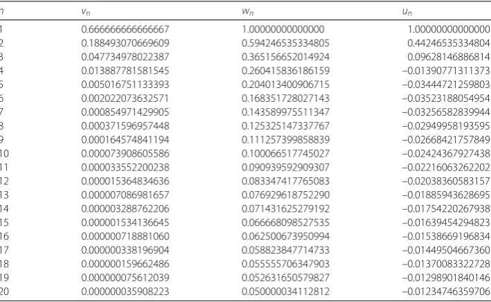
Remark2.18 We do a computational experiment on (2.14) in Remark 2.17 to check the

effectiveness of iterative algorithm (2.4). By using the codes of Visual Basic Six, we get Table 2 and Fig. 2, from which we can see the convergence of{un},{vn}, and{wn}.

2.3 Applications to minimization problems

Leth:E→(–∞, +∞] be a proper convex, lower-semicontinuous function. The

subdif-ferential∂hofhis defined as follows:∀x∈E,

∂h(x) =z∈E∗:h(x) +y–x,z ≤h(y),∀y∈E.

Theorem 2.19 Let E,S,{εn},{sn},{τn},and{αn}be the same as those in Corollary2.3.Let h:E→(–∞, +∞]be a proper convex,lower-semicontinuous function.Let{un}be

gener-Table 2 Numerical esults of{un},{vn}, and{wn}with initialu1= 1.0

n vn wn un

1 0.666666666666667 1.00000000000000 1.00000000000000

2 0.188493070669609 0.594246535334805 0.442465353348047

3 0.047734978022387 0.365156652014924 0.096281468868147

4 0.013887781581545 0.260415836186159 –0.01390771311373

5 0.005016751133393 0.204013400906715 –0.03444721259803

6 0.002022073632571 0.168351728027143 –0.03523188054954

7 0.000854971429905 0.143589975511347 –0.03256582839944

8 0.000371596957448 0.125325147337767 –0.02949958193595

9 0.000164574841194 0.111257399858839 –0.02668421757849

10 0.000073908605586 0.100066517745027 –0.02424367927438

11 0.000033552200238 0.090939592909307 –0.02216063262202

12 0.000015364834636 0.083347417765083 –0.02038360583157

13 0.000007086981657 0.076929618752290 –0.01885943628695

14 0.000003288762206 0.071431625279192 –0.01754220267938

15 0.000001534136645 0.066668098527535 –0.01639454294823

16 0.000000718881060 0.062500673950994 –0.01538669196834

17 0.000000338196904 0.058823847714733 –0.01449504667360

18 0.000000159662486 0.055555706347903 –0.01370083322728

19 0.000000075612039 0.052631650579827 –0.01298901840146

Figure 2Convergence of{un},{vn}, and{wn}

ated by ⎧ ⎪ ⎪ ⎪ ⎪ ⎪ ⎪ ⎪ ⎪ ⎪ ⎪ ⎪ ⎪ ⎪ ⎪ ⎪ ⎪ ⎪ ⎨ ⎪ ⎪ ⎪ ⎪ ⎪ ⎪ ⎪ ⎪ ⎪ ⎪ ⎪ ⎪ ⎪ ⎪ ⎪ ⎪ ⎪ ⎩

u1∈E, ε1∈E,

vn=arg minz∈E{h(z) +₂1_snz2–_s1_nz,J(un+εn)},

wn=J–1[αnJun+ (1 –αn)JSvn],

V1=W1=E,

Vn+1={z∈E:vn–z,J(un+εn) –Jvn ≥0} ∩Vn,

Wn+1={z∈Vn+1:ϕ(z,wn)≤αnϕ(z,un) + (1 –αn)ϕ(z,vn)} ∩Wn,

Un+1={z∈Wn+1:u1–z2≤ PWn+1(u1) –u12+τn+1},

un+1∈Un+1, n∈N.

Then

(1) ifvn=un+εnandwn=J–1[αnJun+ (1 –αn)J(un+εn)]for alln∈N,then

un+εn∈N(∂h)∩F(S).

(2) IfN(∂h)∩F(S)=∅andinf_nsn> 0,then the iterative sequence

un→yo=P∞_n=1Wn(u1)∈N(∂h)∩F(S),asn→ ∞.

Proof Similar to [11],vn=arg minz∈E{h(z) + ₂1_snz2– _s1_nz,J(un+εn)}is equivalent to 0∈∂h(vn) +_s1_nJun–_s1_nJ(un+εn). Thenvn= (J+sn∂h)–1J(un+εn). So, Corollary 2.3 ensures the desired results.

This completes the proof.

Theorem 2.20 We only do the following changes in Theorem2.19:wn=J–1[αnJu1+ (1 – αn)JSvn]and Wn+1={z∈Vn+1:ϕ(z,wn)≤αnϕ(z,u1) + (1 –αn)ϕ(z,vn)} ∩Wn.Then,under

the assumptions of Corollary2.6,we still have the result of Theorem2.19.

Acknowledgements

Competing interests

The authors declare that they have no competing interests.

Authors’ contributions

All authors contributed equally to the manuscript. All authors read and approved the final manuscript.

Author details

1_{School of Mathematics and Statistics, Hebei University of Economics and Business, Shijiazhuang, China.}2_{Department of}

Mathematics, Texas A&M University-Kingsville, Kingsville, USA.

Publisher’s Note

Springer Nature remains neutral with regard to jurisdictional claims in published maps and institutional affiliations.

Received: 1 February 2018 Accepted: 16 February 2018 References

1. Takahashi, W.: Nonlinear Functional Analysis. Fixed Point Theory and Its Applications. Yokohama Publishers, Yokohama (2000)

2. Agarwal, R.P., O’Regan, D., Sahu, D.R.: Fixed Point Theory for Lipschitz-Type Mappings with Applications. Springer, Berlin (2008)

3. Pascali, D., Sburlan, S.: Nonlinear Mappings and Monotone Type. Sijthoff and Noordhoff, The Netherlands (1978) 4. Alber, Y.I.: Metric and generalized projection operators in Banach spaces: properties and applications. In: Kartsatos,

A.G. (ed.) Theory and Applications of Nonlinear Operators of Accretive and Monotone Type. Lecture Notes in Pure and Applied Mathematics, vol. 178, pp. 15–50. Dekker, New York (1996)

5. Zhang, J.L., Su, Y.F., Cheng, Q.Q.: Simple projection algorithm for a countable family of weak relatively nonexpansive mappings and applications. Fixed Point Theory Appl.2012, Article ID 205 (2012)

6. Zhang, J.L., Su, Y.F., Cheng, Q.Q.: Hybrid algorithm of fixed point for weak relatively nonexpansive multivalued mappings and applications. Abstr. Appl. Anal.2012, Article ID 479438 (2012)

7. Matsushita, S., Takahashi, W.: A strong convergence theorem for relatively nonexpansive mappings in a Banach space. J. Approx. Theory134, 257–266 (2005)

8. Liu, Y.: Weak convergence of a hybrid type method with errors for a maximal monotone mapping in Banach spaces. J. Inequal. Appl.2015, Article ID 260 (2015)

9. Su, Y.F., Li, M.Q., Zhang, H.: New monotone hybrid algorithm for hemi-relatively nonexpansive mappings and maximal monotone operators. Appl. Math. Comput.217, 5458–5465 (2011)

10. Wei, L., Tan, R.: Iterative schemes for finite families of maximal monotone operators based on resolvents. Abstr. Appl. Anal.2014, Article ID 451279 (2014). https://doi.org/10.1155/2014/451279

11. Wei, L., Cho, Y.J.: Iterative schemes for zero points of maximal monotone operators and fixed points of nonexpansive mappings and their applications. Fixed Point Theory Appl.2008, Article ID 168468 (2008)

12. Wei, L., Su, Y.F., Zhou, H.Y.: Iterative convergence theorems for maximal monotone operators and relatively nonexpansive mappings. Appl. Math. J. Chin. Univ. Ser. B23(3), 319–325 (2008)

13. Klin-eam, C., Suantai, S., Takahashi, W.: Strong convergence of generalized projection algorithms for nonlinear operators. Abstr. Appl. Anal.2009, Article ID 649831 (2009)

14. Wei, L., Su, Y.F., Zhou, H.Y.: Iterative schemes for strongly relatively nonexpansive mappings and maximal monotone operators. Appl. Math. J. Chin. Univ. Ser. B25(2), 199–208 (2010)

15. Inoue, G., Takahashi, W., Zembayashi, K.: Strong convergence theorems by hybrid methods for maximal monotone operator and relatively nonexpansive mappings in Banach spaces. J. Convex Anal.16(16), 791–806 (2009) 16. Mosco, U.: Convergence of convex sets and of solutions of variational inequalities. Adv. Math.3(4), 510–585 (1969) 17. Tsukada, M.: Convergence of best approximations in a smooth Banach space. J. Approx. Theory40, 301–309 (1984) 18. Kamimura, S., Takahashi, W.: Strong convergence of a proximal-type algorithm in a Banach space. SIAM J. Optim.

13(3), 938–945 (2012)