Differential Gene Expression Analysis of Lung
Cancer Genes of Human and Mouse Using Cluster
G. Anitha Mary1, Prof G. Anjan Babu2
1Asst. Prof, Dept. of MCA, Loyola Academy Degree & PG College, Old Alwal, Secunderabad-10, India, Research Scholar (Ph. D. -
Part-time) Sri Venkateswara University Tirupati.
2Professor & Head, Dept. of Computer Science, Sri Venkateswara University, Tirupati, Chittoor District, A.P, India
Abstract -Phylogenetic trees symbolizes the progression relationship between biological genre and organisms. The construction of phylogenetic trees support on the similarities or dissimilarity of their physical or inherited features. Accepted dawns of constructing phylogenetic trees mainly focus on substantial characteristics. The current appropriation of high-throughput knowledge has advanced to buildup of large quantity of biological data, which in turn enhance the approach of biological studies in a mixture of approaches. This work is mainly focus on constructing the phylogentic tree for Lung cancer genes of Mouse based on experimental values. Here to construct the phylogenetic tree by applying the cluster and by using JavaTree approaches on several genes differential expressed data. These results are shown the better evolutionary relationship among the Lung cancer genes biological datasets proving that similarity with Human lung cancer genes.
Keywords-Cancer, Cluster, Lungs, Oncogenes, Proteins
I. INTRODUCTION
A phylogenetic tree is a vivid demonstration of the completion connections of genus, and the phylogenetic trees reserve surrounded by the species replicate the closeness of evolutionary relationships. Conventional construction of phylogenetic trees was essentially based on physical similarities and diversity. Yet, the procedure of the deepness has been changed because of the production of large amounts of biological data. For ex, high-throughput sequencing expertise have generated genome sequences in more thousand organisms. Basically the genomic sequence is a thread of four unlike kinds of nucleotides (A, C, G and T), with the length from hundreds of thousands to millions. Broadly it has been time-honored that the genomic sequences are extremely analogous for evolutionary closed organisms, but not similar for evolutionary apart organisms. So, genomic sequences have been broadly used for building phylogenetic trees.
The building of phylogenetic trees by means of genomic sequences does have a number of issues. The genomic sequences are frequently lengthy so comparison genomic sequences from end to end species for building phylogenetic trees is computationally costly. On the other hand, living organisms in a small position frequently swap over their genetic materials every other, also recognized as straight gene transfer, making it harder to conclude evolutionary relationships based on genomic sequences only. Additionally, present genomic sequence likeness measurement cannot truly reveal evolutionary relationships across the species. So, it is better to use other data and procedures to report true relationships.
Allelic loss of the p16 tumor suppressor gene occurs in approximately 50% of mouse lung adenocarcinomas [9]. Allelic of chromosomes 1, 4, 11, 12, and 14 are frequently associated with mouse lung tumor development [9–11]. Recently, mouse lung tumor susceptibility loci have been linked to chromosomes 6, 9, 17, and 19. Those linked to lung tumor resistance have been linked to chromosomes 4, 11, 12, and 18 [3]. Detection of mutations or LOH in specific oncogenes and tumor suppressor genes has been the focus in examining for genetic alterations in tumors. Many global procedures have newly implemented. These include CGH analysis, which allows one to examine for gene removal or amplification, and proteomics, which permits to develop of protein levels. The advantage of cDNA microarrays to find change gene evaluation in the process of neoplastic process which has generated the large quantity of struggle till date. In specific, high-density oligonucleotide arrays and high density cDNA glass slide arrays have been widely used in profiling gene explanation in human and cavy tumor tissues.
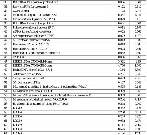
A. Description of Lung Cancer genes data set
S. No. Gene Normal Tumour
1 mRNA for translational controlled 40 -kDa polypeptide p40
0.732 1.548
2 Homo putative transcription factor CA150 0.046 0.194
3 45S pre –rRNA 23.31 79.67
4 mRNA for cysteinyl -tRNA synthetase 0.017 0.071
5 mRNA for pancortin - 1 and – 3 0.014 0.036
6 Serine hydrolase - like ( Serhl ) Mrna 0.025 0.065
7 Human hypothetical protein FLJ11240 0.026 0.057
8 Gene for fibrinogen A-a- chain 0.040 0.179
9 mRNA for erk – 1 0.286 0.566
10 JAK- 1 protein 0.029 0.153
11 Neuronal guanine nucleotide exchange factor 0.016 0.075
12 Zinc finger protein 96 ( Zfp96 ) mRNA 0.020 0.098
13 BALB/ c conserved CHUK mRNA 0.209 0.431
14 mRNA for a- adaptin (C) 0.077 0.264
15 T- cell transcription factor NFAT1 isoform A mRNA 0.034 0.101
16 MCH class I heavy – chain precursor (H- 2D( k ) ) mRNA 2.691 7.093 17 MCH class I heavy – chain precursor (H- 2K( k ) ) mRNA 0.275 1.122
18 Complement component C3 gene, 5’end 0.141 0.887
19 10 -Day - old male pancreas cDNA 0.506 0.443
20 11 -Day embryo cDNA 0.41 0.546
21 13 -Day embryo liver cDNA 1.72 1.227
22 α- Globin mRNA 0.011 0.355
23 β - Globin major gene 0.186 0.602
24 CA IV gene 0.007 0.006
25 ALDH II mRNA 0.076 0.063
26 Growth factor – inducible immediate - early gene, cyr61 0.093 0.018
27 Paroxanase (PON- 1 ) mRNA 0.093 0.027
28 Homo sapiens glucose - regulated protein 0.012 0.07
29 Hybridoma 12A1 immunoglobulin heavy - chain mRNA 0.131 0.026
30 Rat Ras GTPase -activating protein 0.03 0.013
31 H. sapiens TNFa- stimulated ABC protein 0.073 0.063
33 Rat mRNA for ribosomal protein L18a 0.056 0.041
34 Lsp - s mRNA for lysozyme P 0.122 0.116
35 CC10 protein 1.122 0.413
36 Mitochondrial genes for transfer RNA 6.237 4.441
37 Mouse surfactant protein -A (SP-A) 0.079 0.118
38 Rat mRNA for surfactant protein –B 0.401 0.661
39 Pulmonary surfactant protein SP-C 0.014 0.106
40 mRNA for sulfated glycoprotein 0.022 0.062
41 Serine proteinase inhibitor 6 (SPI6) 0.072 0.37
42 a- 1 Protease inhibitor 2 mRNA 0.013 0.037
43 Human mRNA for KIAA0183 0.018 0.082
44 Human mRNA for KIAA0187 0.028 0.391
45 Homolog of D. melanogaster flightless I 0.082 0.492
46 CYP2C40 0.006 0.065
47 RIKEN cDNA 2500002L14 gene 3.322 1.26
48 RIKEN cDNA 5730403B10 gene 4.768 1.693
49 Brain cDNA, clone MNCb- 5704 10.66 3.399
50 Adult male testis cDNA 5.731 2.643
51 0 -Day neonate skin cDNA 6.623 2.317
52 10 -Day embryo cDNA 0.127 0.043
53 Mus musculus proline 4 - hydrosylase a- 1 polypeptide (P4ha1 ) 0.575 0.183
54 M. musculus similar to KIAA1711 0.379 0.055
55 Mouse DNA sequence from clone RP23- 39409 on chromosome 11 0.379 0.046
56 M. musculus hypothetical protein MGC25836 0.254 0.13
57 H. sapiens chromosome 18, clone RP11-749G1 0.363 0.047
58 LRG1# 0.252 0.121
59 LRG2# 2.268 1.09
60 LRG3# 8.239 3.228
61 LRG4# 0.932 0.474
62 LRG5# 6.114 3.16
63 LRG6# 8.576 2.903
[image:4.612.54.561.76.542.2]64 LRG7# 46.64 17.38
Table 1: Gene names and its experimental values
B. Data Processing
The flow chart of our approach is outlined in Figure 1, and the detailed description of every step is presented as follows and it has three steps.
Figure 1: Data Process Load the genes
Take the gene experimental values
[image:4.612.140.406.610.716.2]1) Load the genes: For the initial stage, open the NCBI and extract the names of the genes i.e. their accession numbers in database.
2) To obtain the Result values: The experimental values from the results of Lung Cancer genes. The values are indicating the distinct values in distinct experiments.
3) Store the values obtained from experiments: The experimental values are preserved in excel sheet for further calculation of cluster analysis. Save the values only in Button-Delimited format, because it gives correct outputs in analysis.
II. CLUSTERINGALGORITHM
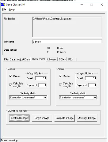
[image:5.612.179.510.256.621.2]Clustering is an unendorsed culture algorithm that finds the concealed arrangement in the unlabeled data. In this work, the filtered values, adjust the data values, apply the hierarchical procedure, k-means algorithm, self-organizing maps (SOM), and finally apply the Principal Component Analysis (PCA) for avoid the unwanted values, adjust the data with help of log transform, for clustering genes and arrays with hierarchical clustering by centroid linkage, to organize the genes with k-means algorithm, calculate the SOMs and PCA analysis [9]. The results were visualized by Java Tree View [10] and scatterplot.
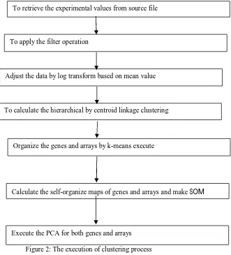
Figure 2: The execution of clustering process
III.RESULTS
A. Applying Filter For the Loaded Data
The initial stage in using Cluster is to link the data. Directly, Cluster reads button-delimited text files only in a specific format. Such button-delimited text files can be created and exported in a standard spreadsheet program Ex. Microsoft Excel.
To retrieve the experimental values from source file
To apply the filter operation
Adjust the data by log transform based on mean value
To calculate the hierarchical by centroid linkage clustering
Organize the genes and arrays by k-means execute
Calculate the self-organize maps of genes andarraysand makeSOM
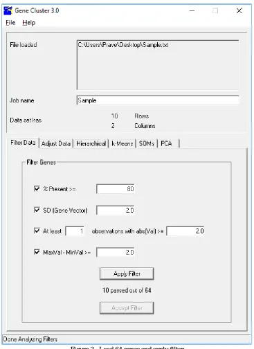
Figure 3 : Load 64 genes and apply filter
The Filter Data button allows to delete genes that do not have certain desired properties from your dataset. The directly available properties can be used for filter data
1) % Present >= X. This deletes all genes that have lacking in values in greater than (100-X) percent of the columns. 2) SD (Gene Vector) >= X. This deletes all genes that have standard deviations of observed values less than X.
3) At least X Observations with abs (Val) >= Y. This deletes all genes that do not have at least X observations with absolute values greater than Y.
These are fairly self-explanatory. When filter button pressed, the filters are not immediately applied to the dataset. In order to accept the filter, press Accept button, if not no changes are made.
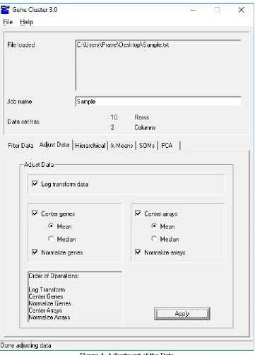
[image:7.612.127.488.133.635.2]B. Adjustment of the data
Figure 4: Adjustment of the Data
From the Adjust Data button, a number of operations that can be calculated that change the basic data in the imported table. These operations include following:
1) Log Transform Data: replace all data values x by log2 (x).
3) Center arrays [mean or median]: Subtract the column-wise mean or median from the values in every column of data, so that the mean or median value of every column is 0.
4) Normalize genes: Multiply all values in every row of data by a scale factor S so that the sum of the squares of the values in every row is 1.0 (a separate S is computed for every row).
5) Normalize arrays: Multiply all values in every column of data by a scale factor S so that the sum of the squares of the values in every column is 1.0 (a separate S is computed for every column).
These operations are not associative, so the order in which these operations is applied is very important, and you should consider it carefully before you apply these operations. The order of operations is (only checked operations are calculated):
1) Log transform all values.
2) Center rows by subtracting the mean or median. 3) Normalize rows.
4) Center columns by subtracting the mean or median. 5) Normalize columns.
C. Log Transformation
The Ratio measurements are most naturally processed in log space. Thus mathematical operations that use the difference between values would think that the 2-fold up change was twice as significant as the 2-fold down change. In log space (we use log base 2 for simplicity) the data points become 0, 1.0, -1.0.With these values, 2-fold up and 2-fold down are symmetric about 0.
D. Mean / Median Centering
For every gene, you have a series of ratio values that are relative to the expression level of that gene in the reference sample. Since the reference sample really has nothing to do with your experiment values, you want your analysis to be independent of the amount of a gene present in the reference sample. This is achieved by adjusting the values of every gene to reflect their variation from some property of the series of observed values such as the mean or median. This is what mean and/or median centering of genes does. Centering makes less sense in experiments where the reference sample is part of the experiment, as it is many time courses. Centering the data for columns/arrays can also be used to delete certain types of biases. Mean or median centering the data in log-space has the effect of correcting the bias, although it should be noted that an assumption is being made in correcting the bias, which is that the average gene in a given experiment is expected to have a ratio of 1.0 (or log-ratio of 0).
E. Normalization
Normalization sets the magnitude (sum of the squares of the values) of a row/column vector to 1.0. Most of the distance metrics used by Cluster work with inside the normalized data vectors, but the data are output as they were really entered.
This results in a log-transformed, median enhanced (i.e. for every row and column median values are close to zero) and normal (i.e. for every row and column magnitudes are close to 1.0) dataset. After calculating these operations, dataset should be saved.
F. Hierarichical Clustering
The Hierarchical Clustering button allows you to calculate hierarchical clustering on the given data. This is a powerful and helpful procedure for analyzing all sorts of huge genomic datasets. Cluster at present calculates four types of binary, agglomerative, hierarchical clustering. The core idea is to group a set of elements (genes or arrays) into a tree, where elements are combined by very short branches if they are very similar to every other, and by increasingly longer branches as their similarity decreases. The initial step in hierarchical clustering is to find the distance matrix between the gene expression data. After matrix distances is computed then, the clustering begins. Agglomerative hierarchical processing consists of repeated cycles where the two nearing remaining elements (i.e. smallest distance) are combined by a node/branch of a tree, with the length of the branch set to the distance between the combined elements. The two combined elements are deleted from list of elements being processed and replaced by an element that represents the new branch. The distances between this new element and all other remaining elements are computed, and the process is continued until an element retained.
using the same similarity metric as was used to calculate the initial similarity matrix. The vector is the average of the vectors of all original elements (Ex. genes) contained within the pseudo-element. Thus, when a new branch of the tree is formed combining group a branch with 5 elements and an original element, the new pseudo-element is assigned a vector that is the average of the 6 vectors it contains, and not the average of the two combined elements
2) Single Linkage Clustering: Single Linkage Clustering is the process of calculating the distance between two elements x and y. It is the minimum of all pairwise distances between elements contained in x and y. Unlike centroid linkage clustering, in single linkage clustering no further distances need to be computed once the distance matrix is done.
3) Complete Linkage Clustering: Complete Linkage Clustering is the process of calculating the distance between two elements x and y. It is the maximum of all pairwise distances between elements contained in x and y. As in single linkage clustering, no other distances need to be computed once the distance matrix is done.
[image:9.612.124.490.230.709.2]4) Average Linkage Clustering: Average linkage clustering is the process of calculating the distance between two elements x and y. It is the mean of all pairwise distances between elements contained in x and y.
5) Output Files: Cluster results in three output files for every hierarchical clustering run. The root filename of every file Sample (current work) i.e. whatever text you enter into the Job Name dialog box. When you load a file, Jo is set to the root filename of the input file. The three output files are ‘Sample.cdt’, ‘Sample.gtr’, ‘Sample.atr’ i.e. Sample.cdt, Sample.gtr, Sample.atr. The ‘.cdt’ (for clustered data buttoned) file contains the original data with the rows and columns reordered based on the clustering result. It is the same format as the input files, except that an additional column and/or row is added if clustering is calculated on genes and/or arrays. This additional column/row contains a unique identifier for every row/column that is linked to the description of the tree structure in the ‘.gtr’ and ‘.atr’ files. The ‘.gtr’ (gene tree) and ‘.atr’ (array tree) files are button-delimited text files that report on the history of node combining in the gene or array clustering (note that these files are produced only when clustering is calculated on the corresponding axis). The ‘.gtr’ and/or ‘.atr’ files are automatically read in Tree View when you open the corresponding ‘.cdt’ file.
[image:10.612.122.491.227.685.2]G. K-MEANS
Figure 6: k-Means clustering
1. The mean vector for all elements in every cluster is computed
2. Elements are reassigned to the cluster whose center is closest to the element
Since the first cluster assignment is random, distinct runs of the k-means clustering algorithm may not give the same end clustering result. To deal with this, the k-means clustering algorithms is continued many times, every time starting from a different beginning clustering. The sum of distances within the clusters is used to relate distinct clustering results. The clustering result with the smallest sum of within-cluster distances is saved for further calculations.
The number of iterations that should be done depends on how difficult it is to find the optimal result, which in turn depends on the number of genes involved. Cluster therefore shows in the status bar how many times the optimal result has been found. If this number is one, there may be a clustering result with an even less sum of within-cluster distances.
The k-means clustering algorithm should then be continued with more trials. If the optimal result is found many times, the result that has been found is likely to have the lowest possible within-cluster sum of distances. We can then assume that the k-means clustering steps are then found the overall optimal clustering result.
[image:11.612.88.490.254.717.2]H. Self-Organizing Maps
Self-Organizing Maps (SOMs) is a procedure of cluster analysis that are likely related to k-means clustering. SOMs were invented in by Teuvo Kohonen in the early 1980s, and have recently been used in genomic analysis. The one-dimensional SOM is used to reorder the elements on whichever axes are selected. The result is similar to the result of means clustering, except that, unlike in k-means clustering, the nodes in a SOM are ordered. This gives to result in a relatively smooth transition between groups.
The options for SOMs are
1) Whether or not, will organize every axis
2) The number of nodes for every axis (the default is n1=4, where n is the number of elements; the total number of clusters is then equal to the square root of the number of elements);
3) The number of iterations to be run.
The output file is of the form ‘Sample_SOM_GXg-Yg_AXa-Ya.txt’, where ‘GXg-Yg’ is included if genes were organized, and ‘AXg-Yg’ is added if arrays were organized. ‘X’ and ‘Y’ represent the dimensions of the corresponding SOM. Up to dual additional files (‘.gnf’ and ‘.anf’) are written having the vectors for the SOM nodes.
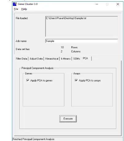
[image:12.612.86.489.258.715.2]I. Principal Component Analysis
Principal Component Analysis (PCA) is a mostly used technique for analyzing multivariate data. In essence, PCA is a coordinate transformation in which every row in the data matrix is written as a linear sum over basis vectors called principal components, which are ordered and chosen such that every maximally explains the remaining variance in the data vectors.
For example, an n×3 data matrix can be represented as an ellipsoidal cloud of n points in three dimensional space. The first principal component is the lengthier axis of the ellipsoid, the second principal component the second lengthier axis of the ellipsoid, and the third principal component is the precise axis. Every row in the data matrix can be rebuilt as a suitable linear combination of the principal components. However, in order to reduce the dimensionality of the data, usually only the most important principal components are retained. The remaining variance present in the data is then regarded as unexplained variance.
The principal components can be found by calculating the Eigen vectors of the covariance matrix of the data. The corresponding eigenvalues determine how much of the variance present in the data is explained by every principal component.
Before applying PCA, typically the mean is deducted from every column in the data matrix. In Cluster, apply PCA to the rows (genes) of the data matrix, or to the columns (microarrays) of the data matrix. In every case, the output consists of two files. When realigning PCA to genes, the names of the output files are ‘Sample_pca_gene.pc.txt’ and ‘Sample_pca_gene.coords.txt’, where the former contains the principal components, and the latter contains the coordinates of every row in the data matrix with respect to the principal components. When realigning PCA to the columns in the data matrix, the respective file names are ‘Sample_pca_array.pc.txt’ and ‘Sample_pca_array.coords.txt’. The original data matrix can be recovered from the principal components and the coordinates.
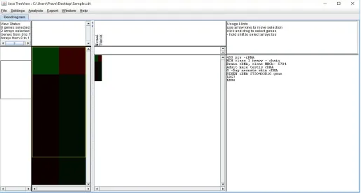
K. Java Tree View
The above clustering is calculated different operations on Lung cancer gene values. In the procedure selected the 64 genes and its values for clustering operations. The procedure provides good results for analyze of phylogenetic tree by using the JavaTree. The output of cluster analysis especially Sample.cdt is helpful in JavaTree for constructing the phylogenetic tree.
[image:13.612.42.557.432.708.2]We have applied Cluster 3.0 on biological value datasets, and used Java Tree View to generate the dendrograms (or phylogenetic trees) for every of the dataset. Figure9show the dendrograms of Lung cancer genes with the lengths of the branches reflecting the length between species. So, precise the branches, the evolutionarily closer the species are, and the lengthier the branches, the evolutionarily many distant the species are.
From the phylogenetic tree in (Figure9), we preserve discover a quantity of fascinating consequences. For ex. the contiguous species by means of human beings is Mus musculus, supposed domicile mouse. To appreciate why these two species stay close, the literature search about the closeness of these two species is done effectively. We found that the genes present in the mouse were also almost all present in humans. Basically, researchers have reported that about 99% of mouse genes have counterparts in humans. The dendrogram outcome for the Lung cancer genes also shows firmly the effectiveness of the approach.
IV.CONCLUSION
In the present work, we have proved that using the sequences of Lung cancer gene revealed the phylogeny of the genes of Mouse and human lung cancers were being clustered and can be further be utilized to make gene networks. The foremost contribution of this study is to demonstrate that with the usage of clustering, the phylogeny of species can be built by a higher-level function. Our experimental results have shown that our approach is pretty accurate in many of cases, firmly indicating that effectiveness of the approach.
REFERENCES
[1] Beckett WS (1993). Epidemiology and etiology of lung cancer. Clin Chest Med 14, 1 – 15. [2] Fielding JE (1985). Smoking: health effects and control ( 1 ). N Engl J Med 313, 491 – 98.
[3] Herzog CR, Lubet RA, and You M (1997). Genetic alterations in mouse lung tumors: implications for cancer chemoprevention. J Cell Biochem Suppl 28 – 29, 49 – 63.
[4] Witschi H, Espiritu I, Maronpot RR, Pinkerton KE, and Jones AD (1997). The carcinogenic potential of the gas phase of environmental tobacco smoke. Carcinogenesis 18, 2035 – 42.
[5] Witschi H, Espiritu I, Peake JL, Wu K, Maronpot RR, and Pinkerton KE (1997). The carcinogenicity of environmental tobacco smoke. Carcinogenesis 18, 575 – 86.
[6] Malkinson AM (1992). Primary lung tumors in mice: an experimentally manipulable model of human adenocarcinoma. Cancer Res 52, 2670s – 76s.
[7] You M, Candrian U, Maronpot RR, Stoner GD, and Anderson MW (1989). Activation of the Ki - ras protooncogene in spontaneously occurring and chemically induced lung tumors of the strain A mouse. Proc Natl Acad Sci USA 86, 3070 – 74.
[8] Re FC, Manenti G, Borrello MG, Colombo MP, Fisher JH, Pierotti MA, Della Porta G, and Dragani TA (1992). Multiple molecular alterations in mouse lung tumors. Mol Carcinog 5, 155 – 60.
[9] Herzog CR, Wang Y, and You M (1995). Allelic loss of distal chromosome 4 in mouse lung tumors localize a putative tumor suppressor gene to a region homologous with human chromosome 1p36. Oncogene 11, 1811 – 15.
[10] Herzog CR, Chen B, Wang Y, Schut HA, and You M (1996). Loss of heterozygosity on chromosomes 1, 11, 12, and 14 in hybrid mouse lung adenocarcinomas. Mol Carcinog 16, 83 – 90.
[11] Hegi ME, Devereux TR, Dietrich WF, Cochran CJ, Lander ES, Foley JF, Maronpot RR, Anderson MW, and Wiseman RW (1994). Allelotype analysis of mouse lung carcinomas reveals frequent allelic losses on chromosome 4 and an association between allelic imbalances on chromosome 6 and K- ras activation. Cancer Res 54, 6257 – 64.