[NORMAL] Combine forecasting method performances for demand forecasting : an exploratory study

JOURNAL OF APPLIED SCIENCES RESEARCH

JOURNAL home page: http://www.aensiweb.com/JASR 2015 March; 11(4): pages 1-6.

Published Online: 15 January 2015. Research Article

Corresponding Author: Rohaizan Ramlan, Department of Production and Operation Management, Universiti Tun Hussein Onn Malaysia.

Tel: +6074533914, Fax: +6074533833, E-mail: [email protected]

Combine Forecasting Method Performances for Demand Forecasting: An

Exploratory Study

1_{Rohaizan Ramlan,} 2_{Raja Zuraidah Raja Mohd Rasi and} 3_{Nur Diyana Mohd Raya}

12_{Department of Production and Operation Management, Universiti Tun Hussein Onn Malaysia} 3_{Department of General Studies, Politeknik Ungku Omar, Malaysia}

Received: 25 November 2014; Revised: 26 December 2014; Accepted: 1 January 2015

© 2015

AENSI PUBLISHER

ABSTRACT

Forecasting is the basis of the decision making process in production. The need to make forecasts in the management and operations is increasing, especially in order to achieve its objectives. Choosing an individual method is more risky than choosing a combination forecast and choosing the individual method may have significantly worse performance than the chosen combination. Hence, the purpose of this exploratory study is to implement and compare the performances of combination forecasting methods. The inventory demand data collected for eight consecutive years. The combine forecast methods used are equal weight combination method and multiple regression combination method. The best forecast method is multiple regressions that provides almost the same demand to the actual product demand and has the lowest total rank of forecast accuracy.

Keywords: Combine Forecasting, Demand Forecasting, Forecasting Method;

INTRODUCTION

Forecasting can be defined as predicting and estimating future demands to provide demand forecasts for company. Many companies do not know their future demands and have to rely on demand forecasts to make decisions in inventory management for both long and short term period. Therefore, forecasting is one of the important measurement methods in decision making [3] as well as an important issue for manufacturing companies [19]. If the forecasting is accurate, major benefits would include reduced safety stock, lower inventory levels and inventory holding costs as well as minimal practice of customer services [21].

Most of the small and medium enterprise (SME) companies in Malaysia determine product demand forecast using judgemental forecast or simple quantitative forecast method such as simple moving average and simple exponential smoothing method [5]. Kerkkanen et al., [20] indicated that the imitation of concepts, targets and principle of forecasting method among consumer products risk for unrealistic accuracy targets and deceptive error measures. Therefore, special characteristics should be addressed and understood before any techniques or approaches are applied [20]. This is also supported by Wilson and Keating [33]. According to Chan et al. [6], there may be several causes for inventory problems such as wrong inventory control system,

inadequate management of the system, inaccurate data etc., but a major cause can be the accuracy or lack of it, in the forecasting of future demands. Hibon and Eygeniou [16] stated that, choosing an individual method is more risky than choosing a combination forecast because the individual method may have significantly worse performance than the combination forecast. Thus, the aim of this study is to explore combine forecasting performance with demand forecasting data.

Background of the case study, demand forecasting and selection of methods and forecast accuracy are reviewed in the next section. Following that is the explanation of a comparison of forecasting methods while in the last section some concluding remarks are then attained.

1. Selection of Materials and Methodology:

This study has used the inventory demand data, collected for eight consecutive years. The data includes the sales unit of one product only.

timely and efficient manner, thus maintaining both channel partners and final customers’ satisfaction [25]. According to Heizer et al. [17], organization uses three types of forecasting in their operation planning such as economic forecasting, technology forecasting and demand forecasting.

Forecasting demand is a technique used by companies to determine and allocate their budgets for an upcoming period of time to provide demand forecasts for company. Companies use forecast to make plans and decisions in inventory management both in long and short term period [28]. Demand forecasting is a process to forecast situation and demand flow that might happen in the future. Forecast that relevant to demand is normally used to forecast a period of one to three years forward [31]. It is more oriented in terms of financial issue and forms with the intensive effort in a short period of time [26]. Business plan is made based on the sales goals obtain from the forecasting result. Moreover, demand forecasting is very essential in planning because it plays as an input to the decision making in business [31].

Bates and Granger [4] introduce the Combining Forecast Method which is considered as a successful alternative to using just an individual in forecasting method. It is supported by Dalrymple and Clemen [10], summarized that combining forecasts has been shown to be practical, economical, and useful. Advantages of combine forecasting are; can lead to increased forecast accuracy Clemen, [10], could yield lower forecast error on average [13], improved forecasting accuracy [27], increasing the predictive performance [1] and produce more accurate forecast than individual method [12].

Combining forecast using regression techniques had been suggested by Crane and Crotty [11]. Granger and Ramanathan [14] have pointed out that the conventional forecast combination methods could

be viewed within a regression framework.

Meanwhile, Wilson and Keating [33] suggested that equal weight method can be referred to as a simple averaging combination method or unweighted mean. This method yields the average value of forecasting of the individual forecast that involves as a result. General formula for combination forecast method is shown as below [33].

Combined forecast = 𝑤1𝐹1+𝑤2𝐹2+⋯+𝑤𝑛𝐹𝑛 (2.1)

The weights can be calculated using the formula as below.

𝑤 = 1/n (2.2)

The second method is the combination method using regression analysis. In determining the weights, the formula can be expressed as below. [33].

Combined forecast = a + 𝑊1 (𝐹1) +𝑊2 (𝐹2) (2.3)

2.1 Forecast Measures of Accuracy:

Kerkkanen et al [20] mentioned that different types of forecast error cause different kinds of impact in production planning and inventory management. In order to get better forecast accuracy, selecting the best forecast measurement is essential. Literature provides several different measures for forecast error. Some of the most popular ones are Means Absolute Percentage Error (MAPE), Mean Squared Error (MSE), Cumulative Error and Average Error or Bias [29,9,24]. Lam et al [22] stated that Mean Absolute Percentage Error (MAPE) has become popular as a performance measure in forecasting because the

easiness in terms of interpretation and

understandable. It is also useful for conveying the accuracy of a model to managers or other non-technical users [7]. Taylor et al. [32] found that the relative performance of the RSME methods is a very similar to MAPE. Both are commonly used as error measure in business [18]. According to some authors, measuring forecast errors improves forecast accuracy [24] and the smaller the forecast error is; the more accurate the forecasting method will be [30]. Therefore in this study, all accuracy measurements that have been discussed, applied to find the best forecasting method. There are a few criteria that can be used to select the most suitable forecasting method, which are Mean Absolute Deviation (MAD), Mean Squared Error (MSE), Mean Absolute Percentage Error (MAPE) and Root Mean Squared Error (RMSE).

MAD (Mean Absolute Deviation) measures forecast accuracy by averaging the magnitudes of the forecast errors (the absolute values of the errors).

𝑀𝐴𝐷 = 1

𝑛 𝑌𝑡− 𝑌 𝑡 𝑛

𝑡=1 (2.4)

MSE (Mean Squared Error) historically has been the primary measure used to compare the performance of forecasting methods, mostly due to its computational ease and its theoretical relevance to statistics.

𝑀𝑆𝐸 = 1

𝑛 𝑌𝑡− 𝑌 𝑡

2 𝑛

𝑡=1 (2.5)

MAPE (Mean Absolute Percentage Error) is the average sum of all the percentage errors for a data set taken without any regards to sign [1].

𝑀𝐴𝑃𝐸 = 1

𝑛

𝑌𝑡−𝑌 𝑡 𝑌𝑡 𝑛

𝑡=1 (2.6)

RMSE (Root Mean Squared) is a good measure of prediction accuracy and it is used frequently to measure the differences between values predicted by a model or an estimator and the values actually observed from the thing being modelled or estimated.

𝑅𝑀𝑆𝐸 = 1

𝑛 (𝑌𝑡

𝑛

2.2 Methodology:

Case study is suitable as the research method in this study as Yin [34] stated that case study research method can be defined as an empirical inquiry that investigates a contemporary phenomenon within its real-life context. This is when the boundaries between phenomenon and context are not clearly evident and in which multiple sources of evidence are used. This study used single case study as defined by Yin [34]. Single case study used to confirm or challenge a theory or to represent a unique or extreme case. Moreover, Yin [34] emphasized that single case study ideal for revelatory cases when an observer may have access to a phenomenon that was previously inaccessible.

In this study, documentation of secondary data will be used. Yin [34] stated that documents could be letters, memoranda, agendas, study reports or any items that could be added to the database. The data taken will be the past data kept by the respective company.

Furthermore, Yin [34] stated that data analysis can be done by examining, categorizing, tabulating, testing or combining both qualitative and quantitative evidence to address the initial propositions of a study. The data obtained in this study will be analyzed using ForecastX software. The rationale of ForecastX to be chosen as the software is because it is the family of forecasting tools, capable of

performing the most complex forecast methods and requires only brief learning curve that facilitated immediate, simple and accurate operation regardless of user’s experience [33].

Result and Discussion

There are two comparisons of performances done in this study. The first one is the multiple

regression combination and equal weight

combination which is being compared to forecast accuracy. The value forecast error of RMSE, MAPE, MSE and MAD is compared to determine the accurate forecasting method. Apart from that is the comparison of forecast demand with actual demand. In this case, if the actual has provides almost the same demand to the actual product demand, it shows that the method is more accurate.

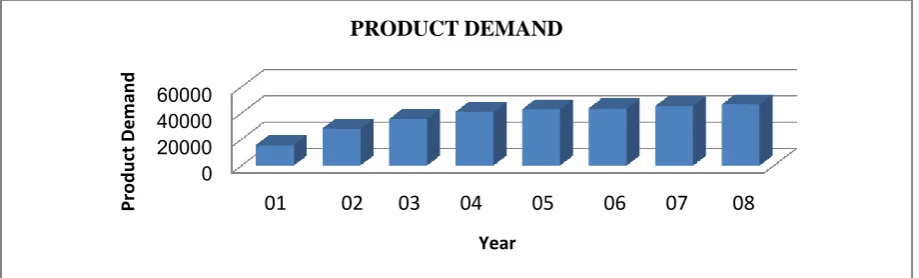
Figure 4.2 shows the product demand for eight consecutive years. Overall, it can be seen that the total product demand from year 1 to year 8 is 298,662 bottles. Based on the graph also, it is shown that there are 15,665 bottles of product demand at year 1, 28,112 bottles at year 2 and 35,414 bottles at year 3. At year 4, there are 40,948 bottles required, 42,828 bottles at year 5 and 43,689 bottles required at year 6. Next, the demand is raised at year 7 to 45,375 bottles and continues expanding to become 46631 bottles at year 8.

Fig. 3.1: Product Demand for Eight Consecutive Years.

3.1 Comparison of Forecast Accuracy and Forecast Method:

The Combine Forecast Method is compared to determine the difference of the performance. Table 4.5 shows the Forecast Accuracy Measurement for forecast methods. Based on the table, the MAPE obtained in Multiple Regression Combine Forecast Method is 5.55%, 143.70 for MAE value, 34,956.87 for MSE and 186.97 for RMSE value. Meanwhile, the forecast accuracy measurement for Equal Weight Combine Forecast is MAE with 526.10, MSE with 431,763.08, RMSE with 657.09 and MAPE with

22.57%. It can be concluded that the Multiple Regression Combine Forecast Method is the best forecast method based on the error of forecast accuracy. It achieved the first place in all of the forecast accuracy measurement.

3.3 Comparison of the Actual Data and Forecast Data:

The purpose of the comparison made is to determine which result forecast techniques have the closer demand data with the actual demand data.

0 20000 40000 60000

2001 2002 2003 2004 2005 2006 2007 2008

Pr

o

d

u

ct

D

e

m

an

d

Year

PRODUCT DEMAND

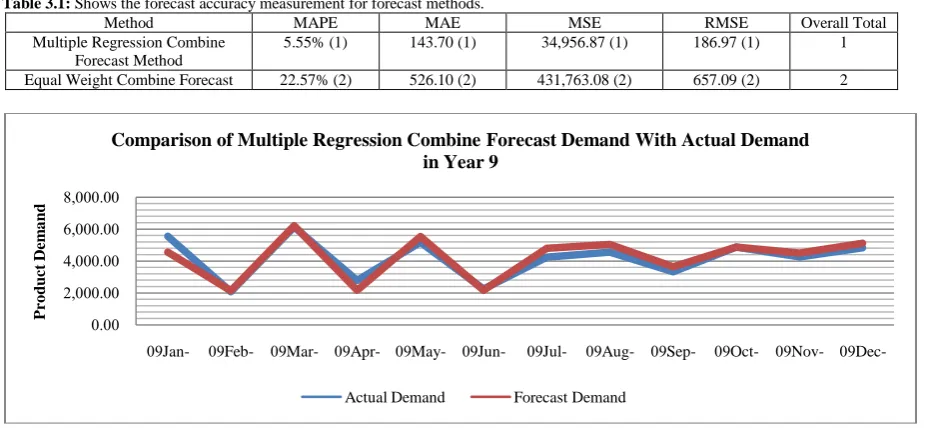
Table 3.1: Shows the forecast accuracy measurement for forecast methods.

Method MAPE MAE MSE RMSE Overall Total

Multiple Regression Combine Forecast Method

5.55% (1) 143.70 (1) 34,956.87 (1) 186.97 (1) 1

Equal Weight Combine Forecast 22.57% (2) 526.10 (2) 431,763.08 (2) 657.09 (2) 2

Fig. 3.2: Comparison of Multiple Regression Combine Forecast Demand with Actual Demand in Year 9.

The figure 4.9 shows the comparison of Multiple Regression Combine Forecast Demand with Actual Demand in Year 9. It can be seen that the critical difference is at January of Year 9 when the actual demand is 5,552 and the forecast demand is 4,645 with the error of 907 bottles. On April of Year 9, the

difference of demand is 613 bottles when actual demand is 2,770 while forecast demand is 2,157 bottles. Moreover, it is shown that the lowest error at February of Year 9 with 9 bottles of error with the actual demand is 2,069 while forecast demand is 2,078 bottles.

Fig. 3.3: Comparison of Equal Weight Combine Forecast Demand with Actual Demand in Year 9.

Figure 4.11 shows the comparison of Equal Weight Combine Forecast Demand with Actual Demand in Year 9. The critical difference is on the February in which the actual demand is 2,059 while the forecast demand is 3,509 with the difference of 1,450 bottles. On the other hand, the smallest difference is in the month of December. The record shows that the difference is only 40 bottles when the actual demand is 4,832 bottles and forecast demand is 4,791 bottles. There is a difference of 1,325 bottles when actual demand is 2,240 while forecast demand is 3,565 bottles in June of Year 9. Based on the result from the comparison of forecast demand and actual demand, it shows that the Multiple Regression

Combine Forecast Method is the best method because of its lowest difference of forecast demand.

Conclusion:

Multiple Regression Combine Forecast Method and Equal Weight Combine Forecast Method have been used for this study to observe the performance of combination forecast methods to forecast the demand of the product. Comparison had been made between equal weight combine forecast method and multiple regression combine forecast method. Overall, it can be said that the best method is Multiple Regression Combine Forecast Method as

0.00 2,000.00 4,000.00 6,000.00 8,000.00

Jan-09 09Feb- 09Mar- 09Apr- 09May- 09Jun- 09Jul- 09Aug- 09Sep- 09Oct- 09Nov- 09

Dec-Pr

o

d

u

ct

D

em

a

n

d

Comparison of Multiple Regression Combine Forecast Demand With Actual Demand in Year 9

Actual Demand Forecast Demand

0.00 1,000.00 2,000.00 3,000.00 4,000.00 5,000.00 6,000.00 7,000.00

Jan-09 09Feb- 09Mar- 09Apr- 09May- 09Jun- 09Jul- 09Aug- 09Sep- 09Oct- 09Nov- 09

Dec-Pr

o

d

u

ct

D

em

a

n

d

Comparison of Equal Weight Combine Forecast Demand With Actual Demand in Year 9

it has the lowest overall total rank value forecast method and the lowest difference of forecast error.

Furthermore, it is suggested that a comparison of performance of time series forecasting and combining forecasting method should be done in future study. Finding from others studies also shows that combining forecast could yield lower forecast error on average [13], improved forecasting accuracy [24] and produce more accurate forecast than individual method [12].

Acknowledgments/Funding/Support:

This research is supported by Ministry of Higher Education of Malaysia (MOHE), under Exploratory Research Grant Scheme (ERGS) to the Office of Research, Innovation, Commercialization and Consultancy (ORRIC), Universiti Tun Hussein Onn Malaysia. Grant number 045/phase I 2013.

Authors’ Contribution:

Rohaizan, Dr. Raja and Nur developed the idea and had an important role in the result, material section and analysis.

Financial Disclosure:

There is no conflict of interest.

References

1. Armstrong, J.S., 2001. Principles of

Forecasting: A Handbook for Researchers and Practitioners Norwell, MA: Kluwer Academic Publishers, 417-439.

2. Armstrong, J.S., 2006. Findings from

Evidence-Based Forecasting: Methods for Reducing Forecast Error. International Journal of Forecasting, 22: 583-598.

3. Yassin, A.M., R. dan Ramlan, 2011.

“Peramalan Terhadap Permintaan Perumahan Awan Kos Rendah” Proceeding of International Seminar on Application of Science Matehmatics 2011.

4. Bates, J.M. and C.W.J. Granger, 1969. The combination of forecasts, Operational Research Quarterly, 20: 451-468.

5. Bon, A.T. and Y.L. Chong, 2009. The

fundamental of demand forecasting in

Inventory Management. Australian Journal of Basic and Applied Sciences, 3(4): 3937-3943. ISSN 1991-8178.

6. Chan, K.C., B.G. Kingsman and H. Wong, 1999. The Value of Combining Forecasts in Inventory Management- A Case Study in Banking. European Journal of Operational Research, 117: 199-210.

7. Chu, F.L., 1998. Forecasting Tourism: A Combined Approach. Tourism Management, 19: 515-520.

8. Chua, Y.P., 2006. Research Method. Malaysia: McGraw-Hill Companies.

9. Chopra, S., P. Meindl, (Eds.) 2001. “Supply Chain Management: Strategy Planning and Operation”, Prentice-Hall Cop., Upper Saddle River, NJ.

10. Clemen, R.T., 1989. Combining forecasts: A

review and annotated bibliography.

International Journal of Forecasting, 5: 559-583.

11. Crane, D.B. and J.R. Crotty, 1967. A two-stage fore-casting model: Exponential smoothing and multiple regression, Management Science, 13: B501-B507.

12. David, F.H. and P.C. Michael, 2002. “Pooling of Forecast”. Econometrics Journal, 5: 1-26. 13. Fuchun Li and G. Tkacz, 2004. Combining

Forecast with Nonparametric Kernel

Regressions, Study in Nonlinear Dynamics & Econometrics, 8(4), article 2.

14. Granger, C.W.J. and R. Ramanathan, 1984. Improved methods of forecasting, Journal of Forecasting, 3: 197-204.

15. Hanke, J.E. and D.W. Wichern, 2009. Business Forecasting. 6th ed. United States of America: Pearson Prentice Hall.

16. Hibon, M. and T. Evgeniou, 2005. To Combine or Not To Combine: Selecting Among

Forecasts and Their Combinations.

International Journal of Forecasting, 21: 15-24. 17. Heizer, J. and B. Render, (7th Eds), 2008. Principles of Operations Management. New Jersey: Pearson, Prentice Hall.

18. Hyndman, R.J. and A.B. Koehler, 2006. “Another look at measures of forecast accuracy”. Journal of Forecasting, pp: 679-688.

19. Kalchschmidt, M., 2007. Demand forecasting practices and performance: Evidence from the GMRG database, Working Papers, Department of Economics and Technology Management, University of Bergamo.

20. Kerkkenen, A., J. Korpela, J. Huiskonen, 2009. “Demand forecasting errors in industrial

context: Measurement and impacts”,

International Journal Production Economics, 118: 43-48.

21. Kerkkenen, A., 2010. “Improving Demand Forecasting Practices In The Industrial Context”. Unpublised Thesis. ISBN 978-952-214-910-7, ISBN 978-952-214-911-4 (PDF), ISSN 1456-4491.

22. Lam, K.F., H.W. Mui and H.K. Yuen, 2001. A Note on Minimizing Absolute Percentage Error in Combined Forecasts. Computers and Operations Research, 28: 1141-1147.

23. Makridakis, S. and M. Hibon, 2000. The

M3-Competition: Results, Conclusions and

Implications. International Journal of Forecasting, 16: 451-476.

24. Mentzer, J.T., M.A. Moon, (Eds), 2005. “Sales

Management Approch, Second Ed.”, Sage Publicaions Inc., Thousand Oaks (CA).

25. Moon, M.A., J.T. Mentzer, C.D. Smith and M.S. Garver, 1998. Seven keys to better forecasting, Business Horizon, pp: 44-52. 26. Raspin, P. and S. Terjesen, 2007. Strategy

making: what have we learned about

forecasting the future? Business Strategy Series, 8(2): 116-121.

27. Robert, L.W. and T.C. Robert, 2004. “Multiple Experts vs. Mutiple Methods: Combining Correclation Assessments”. Decision Analysis, 1(3): 167-176.

28. Ramlan, R., A.A. Siti, R. Umol, 2012. Demand Forecasting In Sme’ S Inventory, Proceedings International Conference of Technology Management, Business and Entrepreneurship 2012 (ICTMBE2012), pp: 792- 796.

29. Russell, R.D., 2000. Operations Management Third ed. Preantice-Hall, Upper Saddle River, NJ.

30. Ryu, K.B.S., 2002. The evaluation of

forecasting Methods at a Institusional Food Service Dining Facility. TexasTEch University: Unpublished Thesis.

31. Shahabuddin, S., 2009. Forecasting automobile sales. Management Research News, 32(7): 670-682.

32. Taylor, J.M., D.J.M. Menezes and M.P.E. Mc Sharry, 2006. “A comparison of Univariate Methods for forecasting Electricity Demand Up to a Day Ahead”. International Journal of Forecasting, 22: 1-16.

33. Wilson, J.H. and B. Keating, 2007. Business Forecasting with Accompanying Excel-Based ForecastX Software. 5th. Ed. New York: McGraw-Hill Companies, Inc.

34. Yin, R.K., 2003. Case Study Research: Design and Methods. Newbury Park, Calif.: Sage. 35. http://people.brunel.ac.uk/~mastjjb/jeb/or/forec