2018 International Conference on Modeling, Simulation and Optimization (MSO 2018) ISBN: 978-1-60595-542-1
Prediction of Maintenance Material Consumption for Aviation Equipment
Using Linear Regression Model
Yan-ming YANG
*, Yue TENG and Rui-li ZHANG
Naval Aviation University Qingdao Campus; Qingdao 266041; China *Corresponding author
Keywords: Aviation equipment, Maintenance material consumption, Linear regression model, Prediction.
Abstract. It is very important to scientifically predict the consumption of aviation equipment maintenance material and to make scientific decisions on aviation equipment maintenance resources and make full use of existing resources to improve maintenance capability. In this paper, aiming at the main influencing factors of material consumption of aviation equipment maintenance, a linear regression prediction model of equipment maintenance material consumption was constructed by using actual statistical sample data. Based on the analysis of examples, the simple linear regression method is used to predict and test the material consumption of aviation equipment maintenance materials. The research results provide a scientific and effective method for forecasting the consumption of aviation equipment maintenance materials.
Introduction
With the development of aviation equipment, more and more complex equipment, maintenance of spare parts required for the variety and quantity are more and more spare parts financing, supply and storage process is also more complex. In this paper, we use linear regression method to forecast the consumption of equipment maintenance material [1]. Regression analysis and forecasting method is based on the analysis of the correlation between independent variables and dependent variables, the regression equation between variables is established, and the regression equation is used as a forecasting method. According to the correlation between independent variables and dependent variables can be divided into linear regression prediction and nonlinear regression prediction. This paper focuses on simple linear regression prediction.
The Principle of Simple Linear Regression Model
In statistics, linear regression is a linear approach for modeling the relationship between a scalar dependent variable y and one or more explanatory variables (or independent variables) denoted X. The case of one explanatory variable is called simple linear regression. For more than one explanatory variable, the process is called multiple linear regression [2-4]. As a commonly used statistical methods and for its principles is clear, model is simple and easy to use, classical linear regression model has been a very wide range of applications in the aviation equipment maintenance and support.
Regression Model
The simple linear regression model is based on the approximate linear relationship between an independent variable and a dependent variable, and is fitted with a linear equation to predict the linear equation. A simple linear regression model is [5]:
y a bx (1)
where y is the forecast object, known as dependent variables or explanatory variables; x is the
influencing factor, known as independent variables or explanatory variables; a, b for the pending
Parameter Estimation
Estimating the parameters a, b in the model, from the point of view of curve fitting, least square
method can be adopted. Suppose you have collected n pairs of data that predict the target y and the
influencing factor x: ( , ) (x yi i i1,..., )n . After analyzing the historical data, assuming a linear
relationship between y and x, you can use the regression model of equation (1). Applying the least
squares method:
1 1 1
2 2
1 1
1 1
n n n
i i i i
i i i
n n i i i i n n i i i i
n x y x y
b
n x x
y b x
a n
or 1 2 1 ( )( ) ( ) n i i i n i ix x y y
b
x x
a y bx
(2)where 1 1 n i i x x n
is called the mean of x;1 1 n i i y y n
is called the mean of y.Model Test
After the regression model is established, whether the model can be used for prediction or not, the model test is also needed. Common statistical tests are standard deviation test and correlation coefficient test.
Standard Deviation Test. Standard deviation s, used to test the accuracy of regression prediction
model, the formula is:
21 1 ˆ 2 n i i i
s y y
n
(3)where ˆyi is the predicted object actual value of the estimated value (or analog value).
The standard deviation s reflects the average error between the estimated and actual values
obtained by the regression prediction model, so the smaller the value of s, the better. The general
requirements of the value of
s y
/
between 10% ~ 15% is appropriate.Correlation Coefficient Test. The correlation coefficient is used to test the significance of the linear correlation between two variables, which is calculated as:
1 2 2 1 1 ( )( ) ( ) ( ) n i i i n n i i i i
x x y y
r
x x y y
(4)It is easy to see that when r = l, the actual value completely falls on the regression line, and y is
completely related to x; when r = 0, y and x are completely uncorrelated; when 0 <r <l, y and x has a
certain correlation. Generally only when r is close to 1, we can describe the relationship between y
and x using a linear regression model. To what extent is r, regression prediction model has practical
significance? The actual test is through the critical correlation coefficient r (usually take a
Application Example Analysis
Problem Description
The monthly statistics of the flight hours of a unit for two years, as shown in Table 1, correspond to the statistical data of the maintenance material consumption, as shown in Table 2. Try to construct a simple linear regression model to predict the maintenance material consumption.
Table 1. Aircraft flight hours statistics in 2015~2016.
Year Jan Feb Mar Apr May Jun Jul Aug Sep Oct Nov Dec
2015 498 191 231 242 403 525 324 370 596 434 518 346
2016 277 235 358 253 538 474 402 458 568 450 398 474
Table 2. Aircraft maintenance material consumption statistics in 2015~2016.
Year Jan Feb Mar Apr May Jun Jul Aug Sep Oct Nov Dec
2015 38 31 39 26 62 50 42 43 61 48 42 51
2016 56 21 29 26 43 56 38 41 66 55 48 35
Predictive Results
[image:3.612.141.475.335.529.2]Using Minitab software regression analysis function to get the following fitted line plot, as shown in Figure 1.
600 500
400 300
200 70
60
50
40
30
20
10
S 3.67196 R-Sq 91.2% R-Sq(adj) 90.8%
Flight hours
Co
ns
um
pt
io
n
qu
an
ti
ty
Regression 95% CI 95% PI
Consumption quantity = 4.173 + 0.09901 Flight hours
Figure 1. Fitted line plot of aircraft flight hours and main maintenance material consumption.
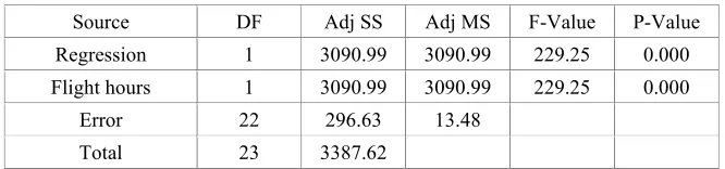
[image:3.612.140.473.624.702.2]Significance Test of Regression Equation. According to Table 3, analyze the results in the ANOVA table first. The P-value corresponding to 229.25 of the F- Value is 0.000 <0.05, so judging the regression equation as a whole is remarkably effective.
Table 3. Analysis of Variance.
Source DF Adj SS Adj MS F-Value P-Value
Regression 1 3090.99 3090.99 229.25 0.000
Flight hours 1 3090.99 3090.99 229.25 0.000
Error 22 296.63 13.48
Total 23 3387.62
explain 90.85% of the variation in maintenance material consumption y, so the model fitting has a
better overall effect.
Table 4. Model Summary.
S R-sq R-sq(adj) R-sq(pred)
3.67196 91.24% 90.85% 89.65%
Significance Test of Regression Coefficient. According to Table 5, the independent variable x
[image:4.612.139.477.192.249.2]coefficient p = 0 <0.05, indicating that the independent variable x is a significant factor.
Table 5. Coefficients.
Term Coef SE Coef T-Value P-Value VIF
Constant 4.17 2.71 1.54 0.138
Flight hours 0.09901 0.00654 15.14 0.000 1.00
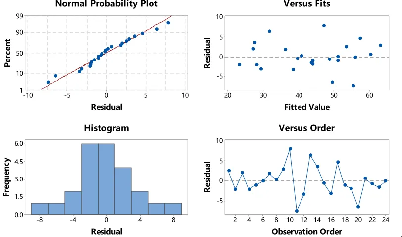
Residual Plots Analysis. Use to examine the goodness of model fit in regression and ANOVA. Examining residual plots helps you determine if the ordinary least squares assumptions are being met. If these assumptions are satisfied, then ordinary least squares regression will produce unbiased coefficient estimates with the minimum variance. Minitab provides the following residual plots (as shown in Figure 2).
10 5
0 -5
-10 99
90
50
10
1
Residual
Pe
rc
en
t
60 50
40 30
20 10
5
0
-5
Fitted Value
Re
si
du
al
8 4
0 -4 -8
6.0
4.5
3.0
1.5
0.0
Residual
Fr
eq
ue
nc
y
24 22 20 18 16 14 12 10 8 6 4 2 10
5
0
-5
Observation Order
Re
si
du
al
Normal Probability Plot Versus Fits
Histogram Versus Order
[image:4.612.104.510.332.571.2]+
Figure 2. Residual plots for aircraft flight hours and main maintenance material consumption.
Residuals Versus Order of Data. This is a plot of all residuals in the order that the data was collected and can be used to find non-random error, especially of time-related effects. This plot helps you to check the assumption that the residuals are uncorrelated with each other. In this example, the residuals fluctuate randomly and are independent of each other.
Residuals Versus Fitted Values. This plot should show a random pattern of residuals on both sides of 0. If a point lies far from the majority of points, it may be an outlier. There should not be any recognizable patterns in the residual plot. For instance, if the spread of residual values tend to increase as the fitted values increase, then this may violate the constant variance assumption. In this example, the graph is normal and the residual is equal variance.
normality assumption may be invalid. In this example, the points are basically in a straight line, and the residuals can be regarded as normal distributions. The residual histogram in the lower left corner can be used to check the distribution of residuals. If you have one or two bars that are farther away from other bars, these may be outliers.
Conclusions
The regression analysis and prediction method is easier to understand, and more widely used. In the actual use process, if the data can be analyzed in detail when selecting specific methods and models, and the observation and analysis of scatter plots can also be more careful, the prediction results will be satisfactory. When the regression prediction method is applied, it is necessary to determine whether there is a correlation between variables. If there is no correlation between the variables, the regression prediction method for these variables will result in the wrong result. When we correctly apply regression analysis, we should pay attention to the qualitative analysis of the relationship between phenomena, avoid any extrapolation of regression prediction, and apply appropriate data. At the same time, the linear regression prediction method proposed in this paper not only applies to the prediction of aviation equipment maintenance material consumption, but also to other equipment indexes or parameters, which provides a scientific method and means for equipment support forecast.
References
[1] Yang, Yanming, W. Wang, and C. Guo. "Forecasting for Air Material Consumption Based on
Winters Exponential Smoothing Model." International Conference on Automation, Mechanical
Control and Computational Engineering 2017.
[2] David A. Freedman. Statistical Models: Theory and Practice. Cambridge University Press. p. 26. (2009)
[3] Rencher, Alvin C.; Christensen, William F., "Chapter 10, Multivariate regression – Section 10.1, Introduction", Methods of Multivariate Analysis, Wiley Series in Probability and Statistics, 709 (3rd ed.), John Wiley & Sons, p. 19, (2012)
[4] Information on https://en.wikipedia.org/wiki/Linear_regression.