Topics in graph colouring and graph structures

(1)

Topics in Graph Colouring

and Graph Structures

David G. Ferguson

A thesis submitted for the degree of

Doctor of Philosophy

Department of Mathematics London School of Economics

(2)

Declaration

I certify that the thesis I have presented for examination for the MPhil/PhD degree of the London School of Economics and Political Science is solely my own work, with the following exceptions:

Chapter 3 is based on joint work with Daniel Kr´al'.

(3)

Abstract

This thesis investigates problems in a number of different areas of graph theory. These problems are related in the sense that they mostly concern the colouring or structure of the underlying graph.

The first problem we consider is in Ramsey Theory, a branch of graph theory stemming from the eponymous theorem which, in its simplest form, states that any sufficiently large graph will contain a clique or anti-clique of a specified size. The problem of finding the minimum size of underlying graph which will guarantee such a clique or anti-clique is an interesting problem in its own right, which has received much interest over the last eighty years but which is notoriously intractable. We consider a generalisation of this problem. Rather than edges being present or not present in the underlying graph, each is assigned one of three possible colours and, rather than considering cliques, we consider cycles. Combining regularity and stability methods, we prove an exact result for a triple of long cycles.

We then move on to consider removal lemmas. The classic Removal Lemma states that, for n sufficiently large, any graph on n vertices containing o(n3) triangles can be made triangle-free by the removal of o(n2) edges. Utilising a coloured hypergraph generalisation of this result, we prove removal lemmas for two classes of multinomials. Next, we consider a problem in fractional colouring. Since finding the chromatic number of a given graph can be viewed as a integer programming problem, it is natural to consider the solution to the corresponding linear programming problem. The solution to this LP-relaxation is called the fractional chromatic number. By a probabilistic method, we improve on the best previously known bound for the fractional chromatic number of a triangle-free graph with maximum degree at most three.

(4)

Acknowledgements

This thesis could not exist without the help and support of numerous people over the last few years. I am hugely indebted to friends, family and colleagues.

Let me begin by thanking my supervisors, Jan van den Heuvel and Jozef Skokan. Thanks to Jan for consistently providing thoughtful feedback on the content and presentation of this thesis and for pointing me in the direction of many interesting problems. Thanks to Jozef for introducing me to stability and regularity in the context of Ramsey Theory and for the many hours spent discussing this thesis over the recent months.

Thanks also to everyone else in the Mathematics Department at the LSE. In particular for helpful discussions, insightful comments and congenial lunchtime chats. I am, of course, also grateful to the department and to the school for financial support received through the LSE research studentship scheme.

I would also like to express my gratitude to the Department of Applied Mathematics at Charles University in Prague and especially to Dan Kr´al'for hosting me as a visitor. Thanks also to Dan for introducing me to fractional colouring and removal lemmas and thanks to my other co-author, Tom´aˇs Kaiser, for sharing ideas and for his efforts in writing up the long case analysis for our fractional colouring paper.

Special thanks go to John Mackay and Peter Allen for taking the time to review an early draft of this thesis and to all my colleagues at the University of Buckingham for their kind support and understanding throughout the last eighteen months.

Too many friends deserve thanks for each to receive a specific mention — their unwa-vering belief in my abilities has sustained me through the most difficult moments of the past few years.

(5)

(6)

Chapter 1

Introduction

This thesis considers a number of problems in graph theory. A graph is an abstract mathematical structure formed by a set of vertices and edges joining pairs of those vertices. Graphs can be used to model the connections between objects; for instance, a computer network can be modelled as a graph with each server represented by a vertex and the connections between those servers represented by edges.

Many problems in graph theory involve some sort of colouring, that is, assignment of labels or ‘colours’ to the edges or vertices of a graph. Such problems fall broadly into two categories: The first type of problem concerns the possibility of assigning colours to a graph while respecting some set of rules; the second concerns the existence of coloured structures in a graph whose colouring we do not control.

The field of graph colouring traces its origins to 1852, when Francis Guthrie observed that a map of the counties of England can be coloured using four colours in such a way that adjacent counties receive different colours. The question of whether this is the case for any such map became known as the Four Colour Problem and is, without doubt, the most well-known problem from the first category above. This problem received much attention over the following century (see, for instance, [Wil03]) before, finally, being answered in the affirmative by Appel and Haken [AH77, AHK77] in 1976.

(9)

such a question should have a finite answer — perhaps, for any size of party, there is a possible list of acquaintances and strangers without such a triad. In fact, it can easily be shown that the answer is six and, as we will see later, that no matter how large a collection of mutual acquaintances or collection of mutual strangers we require, there is a finite size of gathering that will guarantee the existence of one or the other. However, finding the exact answer to this general problem is notoriously difficult.

An interesting feature of many problems in Graph Theory (including the two problems above) is the contrast between the ease with which they may be stated and the appar-ent difficulty of their solution. This contrast is also apparappar-ent in most of the problems considered in this thesis.

Before formally introducing the main themes and problems considered in this thesis, we must give a few key definitions:

1.1

Definitions and notation

The notation used in this thesis is mostly standard and can be found, for instance, in [Bol98], [BM08] and [Die05]. In this section, we give definitions of the objects and concepts we will use most frequently.

Abstractly, a graph is defined by its vertices (which we assume form a finite set) and its edges (each of which joins a pair of distinct vertices). In this thesis we sometimes allow multiple edges between the same pair of vertices. We refer to a graph without such

multi-edges as a simple graph (but usually omit the prefix) and refer to the analogous object in which multi-edges are allowed as amultigraph.

For a given graphG, we useV(G) to denote its vertex set andE(G) to denote its edge set. When it is clear from context which graph is being discussed, we will refer to these sets as simplyV and E respectively.

As is standard, we useKnto denote thecomplete graph onnvertices, that is, the graph onnvertices including all possible edges, and useCn to refer to the cycle onnvertices. Additionally, we use Pn to denote the path on n vertices but will refer to such a path as having lengthn−1, that is, thelength of a pathP, denoted|P|, will be equal to the number of its edges.

(10)

visits every vertex and call such a cycle a Hamiltonian cycle. Analogously, we call a path which visits every vertex a Hamiltonian path.

Given X, a subset of the vertex set of a graph G, we denote by G[X] the graph with vertex set X and edge set {e ∈ E(G) : e ⊆ X}. Similarly, given a pair of disjoint subsets X, Y of the vertex set of a graph G, we use G[X, Y] to denote the subgraph ofG whose edges have one end inX and one end inY.

For a multigraphG, we refer to edges joining the same pair of vertices ascopies of each other. Then, given an edge e, we define the multiplicity of that edge µ(e) to be the number of copies ofepresent inG.

For a (multi)graph G, given a vertex v, we define the degree of that vertex d(v) to be the number of edges (including copies) incident at v. We write δ(G) for the minimum degree, that is, the minimum ofd(v) over the vertices ofG. Similarly, we write ∆(G) for the maximum degree and d(G) for the average degree. We use e(G) to denote _|E(G)_| ande(X, Y) to denote|e(G[X, Y])|. We writed(X, Y) for thedensity of the pair (X, Y), that is,e(X, Y)/|X||Y|.

For a given graphG, we say a set of verticesX_⊆V(G) isindependent ifG[X] contains no edges. Similarly, we define a matching to be a set of independent edges, that is, a collection of pairwise vertex-disjoint edges. Equivalently, for a given graph, a matching is a subgraph in which every vertex has degree one. For a matching M including an edgeuv, we refer to v (resp.u) as theM-mate ofu (resp. v).

For a given graphG, a perfect matching or 1-factor is a matching which spans all the vertices ofGor, equivalently, a spanning subgraph in which every vertex has degree one. Analogously, for a given graph, ak-factor is a spanning subgraph in which every vertex has degreek.

We also consider hypergraphs, that is, structures analogous to graphs in which the edges are permitted to span any number of vertices. Most often, when doing so, we, in fact, considerr-uniformhypergraphs, that is, hypergraphs in which every edge spans exactly

r vertices. Most of the definitions given above carry over from graphs to hypergraphs. In particular, we define d(v),δ(H), ∆(H) in the same way.

(11)

1.2

Graph colouring

In the chapters which follow, we will make use of various notions of colourings of graphs (and hypergraphs). We now define some of these notions and discuss some fundamental results in (proper) graph colouring.

By a colouring of a graph, we mean an assignment of a colour (that is, a label from some list) to either each vertex (avertex-colouring) or each edge (anedge-colouring). A vertex-colouring is calledproper if no two adjacent vertices are assigned the same colour. An edge-colouring is calledproper if no two edges of the same colour meet at a vertex. A (proper)k-colouring is a (proper) colouring using at mostkcolours. Amulticolouring

is a colouring where multiple colours may be assigned to each edge or vertex. Where context permits, we will omit these prefixes so that, for instance, we may refer to a properk-edge-multicolouring simply as a colouring.

Note that, when a small number of colours are being used, it is usual to give them names. In this thesis, the first three colours will always be refered to as red, blue and green (in that order). When a larger number of colours are used, they will be referred to asc1, c2, . . . ck or 1,2, . . . k.

In Chapters 2 and 3 we will make use of colourings without requiring them to be proper. However, it is quite usual for references to graph (and hypergraph) colourings to be taken to refer to proper colourings and indeed we will make use of this notion of colouring in Chapters 4 and 5 and, also, in the remainder of this section.

When colouring a graph, one may ask,

“What is the minimum number of colours required to properly colour a given graph G?”

For vertex-colouring, this minimum is called the chromatic number χ(G) of Gand, for edge-colouring, the chromatic index χ0(G) of G.

At this point, it is worth noting some alternative but equivalent definitions in terms of independent sets. For vertex-colouring, defining acolour class to be the set of vertices assigned a particular colour, we can see that each colour class forms an independent set of vertices and that a properk-vertex-colouring is a partition of the vertices of a graph into k independent sets. Thus, we could define χ(G) to be the minimum k such that there exists a partition of the vertices ofGintokindependent sets. Similarly, defining a

(12)

can see that each colour class forms a matching. Thus, we may view an edge-colouring as a partition and defineχ0(G) to be the minimum ksuch that there exists a partition of the edges ofGintok matchings.

For vertex-colouring, Brooks’ Theorem [Bro41] tells us that we can colour any graphG

using at most ∆(G) + 1 colours and that, for most graphs, ∆(G) colours suffice. More precisely, it tells us that, if G is a connected graph with maximum degree ∆, then

χ(G)≤∆, unlessG is an odd cycle or a complete graph, in which caseχ(G) = ∆ + 1. Given a graph G = (V, E), we define its line graph L(G) to be the graph with vertex set E whose edges are the pairs {e1, e2} ⊆ E which intersect at a vertex in G. Then,

considering the line graph L(G) and applying Brooks’ Theorem gives us the following upper bound for the chromatic index:

χ0(G)≤2∆−1.

However, this upper bound is, in general, not best possible.

Before proceeding, let us note that, when vertex-colouring, the addition of extra copies of any given edge does not alter the possibility or impossibility of colouring a given graph using a given number of colours, since any colouring that is proper for a graph will remain proper if edges are removed or if extra copies of an existing edge are added. However, the same is not true of edge-colourings, since multiple copies of an edge will each require a different colour. Therefore, when discussing edge-colourings, we must specify carefully whether or not to allow multiple copies of a given edge.

Shannon [Sha49] proved the following bound for multigraphs:

χ0(G)_≤ 3₂∆.

Shannon’s bound is the best possible bound of this form, as demonstrated by the Shannon multigraphs shown in Figure 1.1.

Defining µ(G) to be the maximum multiplicity of the edges of G, using a re-colouring argument, Vizing [Viz64] proved the following bound:

(13)

[image:13.595.249.364.92.211.2]

Figure 1.1: Shannon multigraph withχ0(G) = 3₂∆.

which, for simple graphs, reduces to

χ0(G)≤∆(G) + 1,

both of which are best possible.

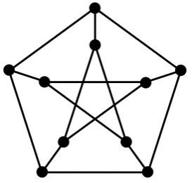
Perhaps the best known, example of a simple graph which cannot be properly edge-coloured using only ∆(G) colours is the Petersen Graph shown in Figure 1.2, which has ∆(G) = 3 butχ0(G) = 4.

Figure 1.2: The Petersen Graph.

Note that, while Vizing tells us that any simple graphG has chromatic index ∆(G) or ∆(G) + 1, the general problem of determiningχ0(G) isNP-complete.

[image:13.595.241.378.410.540.2]

(14)

1.3

Fractional colouring

When considering the chromatic number of certain graphs, one may notice colourings which are best possible (in that they use as few colours as possible) but which are in some sense wasteful. For instance, an odd cycle cannot be properly coloured with two colours but can be coloured using three colours in such a way that the third colour is used only once. Indeed, ifC7 has vertices v1, v2, v3, . . . , v7, then we can colour v1, v3, v5 red,

v2, v4, v6 blue andv7 green.

If, however, our aim is instead to assign multiple colours to each vertex such that adjacent vertices receive disjoint lists of colours, then we could double-colourC7 using five (rather

than six) colours and triple-colour it using seven (rather than nine) colours in such a way that each colour is used exactly three times. Indeed, we could colourvi with colours 3i,3i+ 1,3i+ 2 (mod 7). Thus, asking for the minimum of the ratio of colours required to the number of colours assigned to each vertex gives us a natural generalisation of the chromatic number.

Alternatively, for a graph G = (V, E) we can consider a function w assigning to each independent set of vertices I a real number w(I) ∈ [0,1]. We call such a function a

weighting. The weight w[v] of a vertex v ∈ V with respect to w is then defined to be the sum of w(I) over all independent sets containing v. A weighting w is a fractional colouring of Gif, for each v∈V, w[v]≥1. The size|w|of a fractional colouring is the sum ofw(I) over all independent setsI. Thefractional chromatic number χf(G) is then defined to be the infimum of_|w_|over all possible fractional colourings.

Thus, given a graphG, the problem of findingχf(G) can be viewed as the LP-relaxation of the problem of finding χ(G). Defining I(G) to be the set of independent sets ofG, findingχ(G) is equivalent to solving the following:

minimise X

I∈I w(I),

subject to X I3v

w(I)≥1 for eachv ∈V(G), w(I)_{∈ {}0,1_} for eachI _{∈ I}(G),

(15)

Thus, we can see that, for any graph G, we have

χf(G)≤χ(G).

Also, since χf(G) can be found by solving a linear programming problem with integer coefficients, for any graphG, we know thatχf(G)∈Qand that there exists a colouringw

with |w| = χf(G) such that w(I) ∈ Q∩[0,1] for every I ∈ I. That is, for every

graph G, the infimum in the definition of the fractional chromatic number is attained by a colouring with rational weights.

It can easily be shown that the above two definitions of the fractional chromatic number are equivalent to each other and to a third, probabilistic, definition. It is this third definition which we will make most use of in Chapter 4:

Lemma 1.3.1. Let G be a graph and q a positive rational number. The following are equivalent:

(i) χf(G)≤q;

(ii) there exists an integer N and a multi-set W of at mostqN independent sets in G such that each vertex is contained in exactly N sets from W;

(iii) there exists a probability distribution π on the independent sets of Gsuch that, for

each vertexv, the probability thatvis contained in a random independent set (with

respect to π) is at least 1/q.

Proof.

(i)_⇒(ii): Suppose that χf(G)≤q for someq∈Q. Then, there exists a weighting

w:_{I →}[0,1]

such that P_I₃_vw(I) _≥1 for every v _∈V(G) andP_I_∈_Iw(I) _≤q. As remarked above, we may assume thatw(I)_∈Q∩[0,1] for every I ∈ I.

Then, there exists an integer N such that N w(I)_∈Nfor every I ∈ I. We define W to

include N w(I) copies of each independent set. Thus, _W includes NP_I_∈Iw(I) _≤ N q

(16)

from sufficiently many of those independent sets so as to have every vertex belong to exactlyN sets from W.

(ii)⇒(iii): Suppose there exists an integer N and a multiset W of at most qN inde-pendent sets fromI(G) such that each vertex belongs to exactlyN of the sets from W. Then, define a probability distributionπ:I →[0,1] by

π(I) = (

1/qN ifI _{∈ W},

0 otherwise.

Then, since every vertexv∈V(G) belongs to exactly N members of W, X

I3v

π(I) = 1/q, and X I∈I

π(I) = 1,

as required.

(iii)_⇒(i): Suppose there exists a probability distribution π : _{I →} [0,1] such that P

I3vπ(I)≥1/q and P

I∈Iπ(I) = 1. Then, define a weightingw:I →[0,1] by w(I) = min_{qπ(I),1_}.

Then

X

I3v

w(I)_≥1

for everyv_∈V(G) and X

I∈I

w(I) =X I∈I

min_{qπ(I),1_{} ≤}X I∈I

qπ(I) =q

soχf(G)≤q. 2

(17)

We refer the interested reader to the book of Scheinerman and Ullman [SU97] for more information on fractional colouring.

1.4

Ramsey Theory

Consider the complete graph on N vertices. Suppose we were to colour each of its edges either red or blue and to ask whether this can be done in such a way as to avoid structure in the monochromatic subgraphs induced by the edges of each colour. It is tempting to think that this is possible and that we could find such a colouring which, upon interrogation, would appear to lack structure.

However, this is not the case. For instance, any suchred-blue colouring of the complete graph on six or more vertices will result in either a red or blue triangle (that is, three vertices, say,u, v, w such thatuv, vw, uw are coloured identically). Indeed, consider any vertex v in such a coloured graph along with five of its neighbours, u1, u2, . . . u5. By

the pigeonhole principle, at least three of the edges connectingv to its neighbours, say,

vu1,vu2 andvu3must have the same colour as each other, say, red. Then, consideru1u2,

u2u3 and u1u3. Either one of these three edges is red (giving a red triangle of the form

vuiuj), or they are all blue (giving a blue triangleu1u2u3).

Ramsey’s Theorem [Ram30], essentially tells us that, no matter what structure we re-quire a coloured graph to have in one of its colours, we can guarantee that it will have that structure provided the graph has sufficiently many vertices. We begin by looking at the two-coloured version of the result:

Theorem 1.4.1 ([Ram30]). Given integers n and m, there exists an integer Nr(n, m)

such that, for every integerN ≥Nr(n, m), every red-blue colouring of the complete graph

onN vertices results in the coloured graph containing either a red Kn or a blue Km.

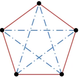
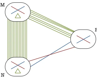
We call the minimum such integer theRamsey Number of (n, m), writtenR(n, m). Notice that our earlier discussion provides a proof thatR(3,3)_≤6 and that the red-blue colouring of K5 shown in Figure 1.3 below shows that R(3,3)> 5, thus completing a

proof thatR(3,3) = 6. Similarly, noting that K2 consists of a single edge, we can see

thatR(2, k) =kfor all k.

(18)

[image:18.595.244.375.90.218.2]

Figure 1.3: A red-blue colouring ofK5 containing no monochromatic triangles.

improved bound for R(n, m). The key argument shows that

R(n, m)_≤R(n₋1, m) +R(n, m₋1)

and proceeds as follows: LetGbe a graph on at leastR(n₋1, m) +R(n, m₋1) vertices. Consider a given vertex v and R(n₋1, m) +R(n, m₋1)₋1 of its neighbours. Then, either there is a setU of at least R(n₋1, m) neighbours ofv with vu coloured red for everyu_∈U or there is a setW of at least R(n, m₋1) neighbours ofvwithvw coloured blue for everyw_∈W. Without loss of generality, assume the latter. Since W contains at leastR(n, m₋1) vertices, it contains either a redKnor a blue Km−1 which, together

withv, forms a blue Km.

Combined with induction and the fact thatR(2, k) =k, this gives an upper bound of

R(n, m)_≤

n+m₋2

n₋1

≤2n+m−2.

For small values ofnandm, the problem of finding the exact value ofR(n, m) is tractable. However, for larger values, things become increasingly more difficult with exact re-sults only known for (n, m) = (2, k),(3,3),(3,4),(3,5),(3,6),(3,7),(3,8),(3,9),(4,4) and (4,5) [Rad94].

Indeed, Joel Spencer [Spe94] recounts some advice given by Erd˝os:

(19)

the aliens...”

Given the difficulty of finding the exact value of R(n, m), results tend to fall into one of two categories: partial results for small values ofn, m and asymptotic results. For a comprehensive overview of results of the first type, see [Rad94].

In terms of asymptotic results, the best known upper bound is due to Conlon [Con09], who proved that there exists a constant C >0 such that

R(n+ 1, n+ 1)_≤n−Clog loglognn

2n n

,

whereas the best known lower bound is due to Spencer [Spe75], who, improving upon a probabilistic argument of Erd˝os [Erd47], proved that

R(n, n)_≥ n√_e22n/2.

Theorem 1.4.1 can be generalised in a number of ways but we will restrict our attention to those extensions which are considered in Chapter 2 of this thesis.

The multicolour Ramsey numberR(n1, n2, . . . , nr) is defined to be the minimumN such that every r-edge-colouring of the complete graph on at least N vertices results in the graph having, as a subgraph, a copy ofKni coloured with colour i, for somei.

Theorem 1.4.2. For every n1, n2, ..., nr, R(n1, n2, . . . , nr) is finite. Moreover,

R(n1, n2, . . . , nr)≤R(R(n1, n2), n3, . . . nr).

Proof. Consider the complete graph on R(R(n1, n2), n3, . . . nr) whose vertices are col-oured with colours 1,2, . . . r. Now, temporarily, cease to distinguish between colours 1 and 2 so that we have anr−1 coloured graph onR(R(n1, n2), n3, . . . nr), which contains either a complete graph onni vertices coloured with colour ifor some 3≤i≤r or con-tains a copy of the complete graph onR(n1, n2) vertices coloured with colours 1 and 2,

which (distinguishing again between colours 1 and 2) contains either a Kn1 coloured

with colour 1 or aKn2 coloured with colour 2. 2

We may also generalise from complete graphs to general graphs as follows: For graphs

(20)

every edge-colouring of KN, the complete graph on N vertices, with up to r colours, results in the graph having, as a subgraph, a copy of Gi coloured with colour i, for somei.

Suppose eachGi hasni vertices. Then, sinceGi is a subgraph ofKni,R(G1, G2, ..., Gr)

is well defined and

R(G1, G2, . . . , Gr)≤R(n1, n2, . . . , nr).

One of the first results in this direction was due to Gerencsér and Gyárfás [GG67] who considered the problem of finding the Ramsey number of a pair of paths and proved that, forn_≤m,

R(Pn, Pm) =m+1₂n−1.

The survey of Radziszowski [Rad94] lists a wealth of results in this direction but we will only mention those which relate directly to the topic of Chapter 2, namely, the Ramsey number of cycles.

The problem of finding the Ramsey number of a pair of cycles was considered in the early 1970s by Bondy and Erd˝os [BE73], Rosta [Ros73] and Faudree and Schelp [FS74] with the second and third sets of authors independently proving the following exact result:

R(Cn, Cm) =                 

6 (n, m) = (3,3),(4,4),

2n₋1 n_≥m_≥3,m odd (n₆= 3), n+1₂m−1 n≥m≥4,n, m even (n6= 4),

max_{n+ 1₂m₋1,2m₋1_} n_≥m_≥4,nodd, m even.

Bondy and Erd˝os noted the difficulty in finding multicolour Ramsey numbers in general, whilst suggesting that, for cycles, the problem should be tractable. They noted that they were

“not able to evaluateR(G1, G2, . . . , Gr) fork >2 even in the case of cycles.”

They did, however, give the following bounds for the r-colour Ramsey number in the case whennis odd:

(21)

and conjectured (see, for instance, [Erd81]) that this lower-bound gives the true value of the Ramsey number.

Recently, there has been renewed interest in these problems. K´arolyi and Rosta [KR01] and Nikiforov and Schelp [NS08] provided new proofs for the two-coloured case. The latter pair utilised stability with the idea being, essentially, to consider the complete graph on slightly fewer than R(Cn, Cm) vertices, to assume that this has a red-blue colouring with no redCnor blueCm and to show that this forces a particular structure which can then be exploited to give a cycle in the larger graph. This idea of a stability proof will be of great use to us in Chapter 2, where we will look at the analogous result for three colours.

1.5

Szemer´

edi’s Regularity Lemma and its applications

Szemer´edi’s Regularity Lemma tells us essentially that any sufficiently large graph can be approximated by the union of a bounded number of random-like bipartite graphs. The earliest version of the result appeared in 1975 in [Sze75] where it was used as a tool in the proof a conjecture of Erd˝os and Tur´an that, for any d >0 and any integerk, any set ofdN integers from_{0,1, . . . , N_}contains a k-term arithmetic progression, provided N

is sufficiently large. The most well known version of the Regularity Lemma for general graphs was later proved in [Sze78].

Recalling the definition of the density of a pair of sets of vertices, that is,

d(X, Y) = e(X, Y) |X_||Y_| ,

we define the concept of a regular pair:

Definition 1.5.1. A pair of disjoint subsets (A, B) of the vertex set of a graph G is

(, G)-regular for some > 0 if, for every pair (A0, B0) with A0 _⊆ A, _|A0_{| ≥} _|A_|, B0 _⊆B, _|B0_{| ≥}_|B_|, we have

d(A0, B0)₋d(A, B)< .

(22)

given any graph on sufficiently many vertices, we can partition the vertices into a bounded number ofclusters such that most pairs of clusters are regular.

Theorem 1.5.2(Szemer´edi’s Regularity Lemma [Sze78]). Given >0andk0a positive

integer, there exists N1.5.2=N1.5.2(, k0) such that the following holds: For all graphs G

with_|V(G)_{| ≥}N1.5.2, there exists a partition Π = (V0, V1, . . . , VK) of V such that

(i) k0 ≤K ≤N1.5.2;

(ii) _|V0| ≤|V|;

(iii) |V1|=|V2|=· · ·=|VK|; and

(iv) all but at most K₂ of the pairs (Vi, Vj) are (, G)-regular.

Note that, for for a given graph Gand a value of, we call a partition (V1, V2, . . . , VK) satisfying (ii)–(iv) above an (, G)-regular partition.

In Chapter 2 , we make use of a coloured version of the Regularity Lemma to define, for a given graph, its reduced graph whose vertices correspond to the clusters arising from the Regularity Lemma and whose edges correspond to the regular pairs. We also make use of a related blow-up lemma, which tells us that an edge in the reduced graph can be ‘blown up’ to a long path in the original graph.

In Chapter 3, we will look at Removal Lemmas, the first and most famous of which is the Triangle Removal Lemma of Ruzsa and Szemer´edi [RS78], which states that a graph onnvertices containingo(n3_{) triangles can be made triangle-free by the removal of}_o₍_n2₎

edges (where we say graph G contains k copies of graph H if G has, as subgraphs, k

graphs isomorphic toH).

A more precise formulation of this result, which was one of the earliest applications of the Regularity Lemma, follows. We also include its proof in full, since the counting required parallels that found in many places in Chapter 2.

Theorem 1.5.3 (The Triangle Removal Lemma [RS78]). For every >0, there exists N1.5.3 = N1.5.3() and δ = δ1.5.3() such that, if G is a graph on n ≥ N vertices with

at most δn3 triangles, then one can remove from G at most n2 edges to obtain a graph

(23)

Proof. Given > 0, we set k0 = 4/. By the Regularity Lemma there exists N =

N1.5.2(/4,4−1) such that, given a graph G on n ≥ N vertices (with fewer than δn3

triangles), there exists a partition Π ofV(G) intoK+ 1 clustersV0, V1, . . . , VK such that

(i) 4/≤K ≤N; (ii) |V0| ≤ 1₄|V|;

(iii) _|V1|=|V2|=· · ·=|VK|; and

(iv) all but at most 1₄ K₂ of the pairs (Vi, Vj) are (1₄, G)-regular.

We then remove fromGany edges (x, y)_∈Xi×Xjsuch that at least one of the following conditions hold:

(i) (Xi, Xj) is not 1₄-regular; (ii) e(Xi, Xj)< ₂1|Xi||Xj|; (iii) x_∈X0;

(iv) Xi =Xj.

Observe that there are at most 1₂(1₄)K2 _{non-regular pairs, giving at most} 1

8K2|V1|2 ≤ 18n2

edges of the first type. By definition, there are at most 1₂n2 _{edges of the second type}

and at most 1₄n2 _{edges of the third type. Finally, there are at most}

K

|V1|

2

≤ 1 2K

_n

K

2

= n

2

2K

edges of the fourth type. Thus, sinceK _≥k0 ≥4/, we have deleted at mostn2 vertices

in total.

Now, suppose that there remains a triangle in G. Since we have removed all edges from within each cluster and all edges intersectingV0, the three vertices of the triangle

(24)

We claim that at most 1₄|X|of the vertices inXhave fewer than 1₄|Y|neighbours inY. Indeed, if this were not the case, these vertices would defineX0 ⊆X with|X0| ≥ 1

4|X|

and e(X0, Y) < 1₄|X0||Y|. However, we know that e(X, Y) ≥ 1

2|X||Y| and by the

definition of a regular pair have

d(X0, Y)−d(X, Y)≤ 1 4,

giving a contradiction. Similarly, we may assume that there are at most 1₄|X|vertices inX with fewer than 1₄|Z|neighbours in Z.

Thus, there are at least (1₋1₂)_|X_|vertices inXwith at least 1₄_|Y_|neighbours inY and at least 1₄_|Z_| neighbours in Z. Given such a vertex, we consider the edges in G[Y, Z] betweenN(x)∩Y andN(x)∩Z. There are at least

2 − 4 4 4

|Y_||Z_|

such edges. Since there are at least (1₋ 1₂)_|X_|such vertices inX, these give rise to at least 1₋ 2 4 3

|X_||Y_||Z_{| ≥}1₋ 2

4

3₍₁₋₎_n

K

3

triangles, giving rise to a contradiction provided

1− 2

4

3₍₁₋₎_n

K

3

> δ.

If > 1₂, the result is trivial. Hence, we may assume that≤ 1₂, in which case

1₋ 2

4

3₍₁₋₎_n

K 3 ≥ 3 4 4 3 ₁ 23 _n K 3 ≥ 1 210 3

K3.

Thus, we may set

δ1.5.3() =

1 210 3 K3

in order to complete the proof. 2

(25)

1.6

Thesis outline

In Chapter 2, combining regularity and stability methods we prove an exact result in Ramsey Theory. For a triple of long cycles of particular parities, we provide an exact answer to the question of how large an underlying three-coloured graph must be in order to guarantee a monochromatic cycle of specified length.

We then move on, in Chapter 3, to consider removal lemmas for equations over finite fields. Utilising a coloured hypergraph generalisation of the Graph Removal Lemma, we prove a removal lemma for two specific classes of multinomials. Specifically, for

X1, X2, . . . Xm subsets of a finite field of of order q, we prove that, if a multinomial of order m of a particular form has o(qm−1) solutions (x1, x2, x3, . . . , xm) with xi ∈ Xi, then we can deleteo(q) elements from each Xi so that no solutions remain.

Next, in Chapter 4, we consider a problem in fractional colouring. By a probabilistic method, we prove that, ifGis a triangle-free graph with maximum degree at most three, then the fractional chromatic number ofG is at most 32/11≈2.909, improving on the best previously known bound. Note that the proof includes a long case analysis which is postponed to the Appendix of this Thesis.

(26)

Chapter 2

The Ramsey number of cycles

Recall that, for graphs G1, G2, G3, the Ramsey number R(G1, G2, G3) is the smallest

integerN such that every edge-colouring of the complete graph on N vertices with up to three colours, results in the graph having, as a subgraph, a copy ofGi coloured with colour i for some i. In this chapter, we will consider the case when G1, G2 and G3

are cycles.

In 1973, Bondy and Erd˝os [BE73] conjectured that, if n >3 is odd, then

R(Cn, Cn, Cn) = 4n−3.

Later, Luczak [ Luc99] proved, that for n odd, R(Cn, Cn, Cn) = 4n+o(n) as n → ∞. Kohayakawa, Simonovits and Skokan [KSS09a], expanding upon the work of Luczak, confirmed the Bondy-Erd˝os conjecture for sufficiently large odd values of n by proving that there exists a positive integern0 such that, for all odd n, m, ` > n0,

R(Cn, Cm, C`) = 4 max{n, m, `} −3.

In the case when all three cycles are of even length, Figaj and Luczak [F L07a] proved the following asymptotic. Defining_hhx_iito be the largest even integer not greater thanx, they proved that, for allα1, α2, α3>0,

R(C_hh_α₁_n_ii, C_hh_α₂_n_ii, C_hh_α₃_n_ii) = 1₂ α1+α2+α3+ max{α1, α2, α3}n+o(n),

(27)

Thus, in particular, for evenn,

R(Cn, Cn, Cn) = 2n+o(n), asn→ ∞.

Independently, Gyárfás, Ruszinkó, Sárközy and Szeméredi [GRSS07] proved a similar, but more precise, result for paths, namely that there exists a positive integer n1 such

that, forn > n1,

R(Pn, Pn, Pn) =   

2n₋1, nodd, 2n−2, neven.

More recently, Benevides and Skokan [BS09] proved that there exists n2 such that, for

evenn > n2,

R(Cn, Cn, Cn) = 2n.

In this chapter, we look at the mixed-parity case, for which, defining _hx_i to be the largest odd number not greater than x, Figaj and Luczak [F L07b] proved that, for all

α1, α2, α3>0,

(i) R(C_hh_α₁_n_ii, C_hh_α₂_n_ii, C_h_α₃_n_i) = max_{2α1+α2, α1+ 2α2,1₂α1+₂1α2+α3}n+o(n),

(ii)R(C_hhα1nii, Chα2ni, Chα3ni) = max{4α1, α1+ 2α2, α1+ 2α3}n+o(n),

asn_{→ ∞}.

Improving on their result, in the case when exactly one of the cycles is of odd length, we prove the following, which is the main result of this chapter:

Theorem A. For everyα1, α2, α3 >0 such that α1 ≥α2, there exists a positive integer

nA=nA(α1, α2, α3) such that, for n > nA,

R(C_hhα1nii, Chhα2nii, Chα3ni) = max{2hhα1nii+hhα2nii−3,

1

2hhα1nii+12hhα2nii+hα3ni−2}.

Additionally, in Section 2.13, we give an outline of the proof of the corresponding result for the case when one of the cycles is of even length and the other two are of odd length. Theorem C. For everyα1, α2, α3>0 such thatα2≥α3, there exists a positive integer

nC =nC(α1, α2, α3) such that, for n > nC,

(28)

2.1

Lower bounds

Our first step in proving Theorem A is to exhibit three-edge-colourings of the complete graph on

max2hhα1nii+hhα2nii − 4, 1₂hhα1nii+1₂hhα2nii+hα3ni − 3

vertices which do not contain any of the relevant coloured cycles, thus proving that

R(C_hh_α₁_n_ii, C_hh_α₂_n_ii, C_h_α₃_n_i)_≥max_{2_hhα1nii+hhα2nii−3, 1₂hhα1nii+₂1hhα2nii+hα3ni−2}.

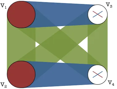
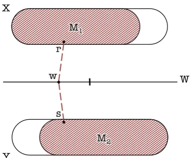
For this purpose, the well-known colourings shown in Figures 2.1 and 2.2 suffice. The graph shown in Figure 2.1 has 2_hhα1nii+hhα2nii−4 vertices divided into four classes

V1, V2, V3 andV4, with

|V1|=|V2|=hhα1nii −1, |V3|=|V4|= 1₂hhα2nii −1,

such that all edges inG[V1] andG[V2] are coloured red; all edges inG[V1, V3] andG[V2, V4]

are coloured blue; all edges in G[V1 ∪V3, V2 ∪V4] are coloured green; and all edges in

G[V3] and G[V4] are coloured red or blue.

V1 V3

[image:28.595.215.405.467.612.2]

V2 V4

Figure 2.1: First extremal colouring for Theorem A.

Since there are no red edges between the vertex classes and each class contains fewer thanhhα1niivertices, the graph has no red cycles of lengthhhα1nii. Also, since there are

(29)

eitherG[V1, V3]∪G[V3] (and, thus, have at least half its vertices inV3) orG[V2, V4]∪G[V4]

(and, thus, have at least half its vertices inV4). Thus, since|V3|,|V4|= 1₂hhα2nii −1, the

graph has no blue cycles of lengthhhα2nii. Finally, since the only green edges belong to

G[V1∪V3, V2∪V4], all green cycles in the graph are of even length. Thus, the graph has

no green cycles of odd length and, in particular, no green cycles of lengthhα3ni.

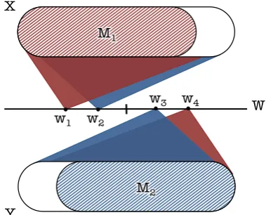
The graph shown in Figure 2.2 has 1₂hhα1nii+1₂hhα2nii+hα3ni −3 vertices, divided into

three classesV1, V2 andV3, with

|V1|= 1₂hhα1nii −1, |V2|= ₂1hhα2nii −1, |V3|=hα3ni −1.

such that all edges in G[V1]∪G[V1, V3] are coloured red; all edges in G[V2]∪G[V2, V3]

are coloured blue; and all edges inG[V1, V2]∪G[V3] are coloured green.

V₁

V2

[image:29.595.213.406.333.475.2]

V₃

Figure 2.2: Second extremal colouring for Theorem A.

Similarly, this graph has no red cycles of length_hhα1nii, no blue cycles of lengthhhα2nii

and no green cycles of length_hα3ni.

Thus, it remains to prove the corresponding upper-bound. To do so, we combine reg-ularity (as used in [ Luc99], [F L07a], [F L07b]) with stability methods using a simillar approach to [GRSS07], [BS09], [KSS09a], [KSS09b].

(30)

2.2

Key steps in the proof

In order to complete the proof of Theorem A, we must show that, fornsufficiently large, any three-colouring ofG, the complete graph on

N = max2hhα1nii+hhα2nii − 3, 1₂hhα1nii+1₂hhα2nii+hα3ni − 2

vertices, will result in either a red cycle on hhα1nii vertices, a blue cycle onhhα2niior a

green cycle on hα3ni vertices.

The main steps of the proof are as follows: Firstly, we apply a version of the Regularity Lemma (Theorem 2.3.1) to give a partition V0 ∪V1∪ · · · ∪VK of the vertices which is simultaneously regular for the red, blue and green spanning subgraphs ofG. Given this partition, we define the three-multicoloured reduced-graphG on vertex setV1, V2, . . . VK whose edges correspond to the regular pairs. We colour the edges of the reduced-graph with all those colours for which the corresponding pair has density above some threshold. Luczak [ Luc99] showed that, if the threshold is chosen properly, then the existence of a matching in a monochromatic connected-component of the reduced-graph implies the existence of a monochromatic cycle of the corresponding length in the original graph. Thus, the key step in the proof of Theorem A will be to prove a Ramsey-type stability result for so-called connected-matchings (Theorem B). Defining aconnected-matching to be a matching with all its edges belonging to the same component, this result essentially says that, for everyα1, α2, α3 >0 such thatα1 ≥α2and every sufficiently largek, every

three-multicolouring of a graph G on slightly fewer than K = max{2α1 +α2,1₂α1 + 1

2α2+α3}kvertices with sufficiently large minimum degree results in either a

connected-matching on at least α1k vertices in the red subgraph of G, a connected-matching on

at least α2k vertices in the blue subgraph of G, a connected-matching on at least α3k

vertices in a non-bipartite component of the green subgraph of G or one of a list of particular structures which will be defined later.

(31)

In the next section, given a three-colouring of the complete graph onN vertices, we will define its three-multicoloured reduced-graph. We will also state and prove a version of the blow-up lemma of Figaj and Luczak, which motivates our whole approach.

In Section 2.4, we will deal with some notational formalities before proceeding in Sec-tion 2.5 to define the structures we need and to give a precise formulaSec-tion of the connected-matching stability result which we shall call Theorem B.

In Section 2.6, we give a number of technical lemmas needed for the proofs of Theorem A and Theorem B. Among these is a decomposition result of Figaj and Luczak which provides insight into the structure of the reduced-graph.

The hard work is done in Sections 2.7–2.8, where we prove Theorem B, and in Sec-tions 2.9–2.12, where we translate this result for connected-matchings into one for cycles, thus completing the proof of Theorem A.

The proof of Theorem B is divided into two parts according to the relative sizes of α1

and α3. Section 2.7 deals with the case when α1 ≥ α3, that is, the case when the

longest cycle has even length. In that case, a combination of the decomposition lemma of Figai and Luczak and some careful counting of edges allows for a reasonably short proof. Section 2.8 deals with the opposite case, which requires a longer proof utilising an alternative decomposition and extensive case analysis.

The final part of the proof of Theorem A is divided into four sub-parts, one dealing with the general setup and three further sections, each dealing with one of the structures that can occur.

Note that Sections 2.3–2.7, 2.9 and 2.10 together give a complete proof for the case where the longest cycle is of even length, allowing the reader to omit sections 2.8, 2.11 and 2.12, while still getting a good flavour of the method of proof.

2.3

Cycles, Matchings and the Regularity Lemma

(32)

Finally, recall that we say such a pair is (, G)-regular for some >0 if, for every pair (A0, B0) withA0 ⊆A,|A0| ≥|A|,B0⊆B,|B0| ≥|B|, we have|d(A0, B0)−d(A, B)|< .

In this chapter, we will make use of a generalised version of Szemer´edi’s Regular-ity Lemma in order to move from considering monochromatic cycles to considering monochromatic connected-matchings, the version below being a slight modification of one found, for instance, in [KS96]:

Theorem 2.3.1. For every > 0 and every positive integer k0, there exists K2.3.1 =

K2.3.1(, k0) such that the following holds: For all graphs G1, G2, G3 with V(G1) =

V(G2) = V(G3) = V and |V| ≥ K2.3.1, there exists a partition Π = (V0, V1, . . . , VK)

of V such that

(i) k0 ≤K ≤K2.3.1;

(ii) |V0| ≤|V|;

(iii) _|V1|=|V2|=· · ·=|VK|; and

(iv) for each i, all but at most K of the pairs (Vi, Vj), 1≤i < j ≤K, are

simultane-ously (, Gr)-regular for r= 1,2,3.

Note that, given > 0 and graphs G1, G2 and G3 on the same vertex set V, we call a

partition Π = (V0, V1, . . . , VK) satisfying (ii)–(iv) (, G1, G2, G3)-regular.

In what follows, given a three-coloured graph G, we will use G1, G2, G3 to refer to its

monochromatic spanning subgraphs. That isG1 (resp. G2, G3) has the same vertex set

asGand includes, as an edge, any edge which in Gis coloured red (resp. blue, green). Then, given a three-coloured graph G, we can use Theorem 2.3.1 to define a partition which is simultaneously regular forG1,G2,G3 and then define the three-multicoloured

reduced-graph_G as follows:

Definition 2.3.2. Given > 0, ξ > 0, a three-coloured graph G = (V, E) and an

(, G1, G2, G3)-regular partition Π = (V0, V1, . . . , VK), we define the three-multicoloured (, ξ,Π)-reduced-graph G= (V,E) by:

V ={V1, V2, . . . , VK},

E=_{ViVj : (Vi, Vj) is simultaneously (, Gr)-regular for r= 1,2,3},

(33)

One well known fact about regular pairs is that they contain long paths. This is sum-marised in the following lemma, which is a slight modification of one found in [ Luc99]: Lemma 2.3.3. For every such that 0 _≤ < 1/600 and every k_≥ 1/, the following holds: LetGbe a bipartite graph with bipartitionV(G) =V1∪V2 such that|V1|,|V2| ≥k,

the pair (V1, V2) is-regular and e(V1, V2)≥1/2|V1||V2|. Then, for every integer `such

that 1 _≤` _≤ k₋21/2_k _{and every} _v0 _∈ _V

1, v00 ∈ V2 such that d(v0), d(v00) ≥ 2₃1/2k, G

contains a path of length 2`+ 1 betweenv0 and v00.

Proof. We begin by considering the case when 1≤`≤ 1₂1/2k.

Suppose there existsU1 ⊆V1of size at leastksuch thatd(u)≤ 2₃1/2kfor everyu∈U1.

By regularity,d(U1, V2) is within ofd(V1, V2).

But

d(V1, V2)≥1/2 and d(U1, V2)< 2₃1/2,

which, since <1/600, gives a contradiction.

Thus, we can discard at mostk vertices from each of V1, V2 to obtainVb1,Vb2 such that

|Vb1|,|Vb2| ≥(1−)k and the subgraph H induced in G by Vb1∪Vb2 has minimum degree

at least 2₃1/2k ₋k _≥ 1₂1/2k+k + 1 (provided k _≥ 1/). We can then greedily construct a pathP =v0v1. . . v2`−2 of length 2`−2 from v0 =v0 ∈Vb1 tov2`−2∈Vb1 such

that v00 _∈/ P. Then, defining W1 ⊆ V1 to be the set of neighbours of v00 in Vb1\P and

W2 ⊆V2 to be the set of neighbours of v2`−2 inVb2\P, we have |W1|,|W2| ≥k. Then,

by regularity,d(W1, W2)≥d(V1, V2)−≥1/2− >0. Thus, there exists an edgew1w2

betweenW1 andW2 which can be used along withv2`−2w1 andw2v00 to extend the path

to length 2`+ 1.

Now, suppose that 1₂1/2k _≤ ` _≤ k₋21/2k and that we have constructed a path

P =v0v1v2. . . v2`−1 from v0 =v0 ∈Vb1 tov2`−1=v00∈Vb2. Consider V1∩P,V2∩P and

suppose we haveW1⊆V1∩P such that|W1| ≥k and every w∈W1 has fewer thank

neighbours in V2\P.

Then, by regularity,

|d(V1∩P, V2\P)−d(W1, V2\P)| ≤ |d(V1∩P, V2\P)−d(V1, V2)|

(34)

and

d(V1∩P, V2\P)> d(V1, V2)−= (1/2−),

but

d(W1, V2\P) =

e(W1, V2\P)

|W1||V2\P| ≤

k_|W1|

|W1||V2\P| ≤

k

|V2\P| ≤ 1 21/2,

which, since_≤1/600, gives rise to a contradiction.

So, all but at most k vertices in V1 ∩ P have at least k neighbours in V2\P and,

similarly, all but at mostkvertices inV2∩P have at leastkneighbours inV1\P. Since

|V1∪P|,|V2∪P| ≥ 1₂1/2k ≥ 2k, there exists i such that vi ∈ V1 ∩P has at least k

neighbours inV2\P (call the set of these neighboursX) andvi+1∈V2∩P has at leastk

neighbours inV1\P (call the set of these neighboursY). The density of (X, Y) is within

of the density of (V1, V2) and so is non-zero. Therefore, there exists an edge xy such

that x _∈ X and y _∈ Y, which can be used to give a path v0v1. . . vixyvi+1. . . v2`−1 of

length 2`+ 1. 2

Recall that we call a matching with all its vertices in the same component of G a

connected-matching and note that we say a connected-matching isodd if the component containing the matching also contains an odd cycle.

The following theorem makes use of the Lemma above to blow up large connected-matchings in the reduced-graph to cycles (of appropriate length and parity) in the orig-inal. This facilitates our approach to proving Theorem A in that it allows us to shift our attention away from cycles to connected-matchings, which turn out to be somewhat easier to find.

Figaj and Luczak [F L07b, Lemma 3] proved a more general version of this theorem in a slightly different context (they considered any number of colours and any combination of parities and used a different threshold for colouring the reduced-graph):

Theorem 2.3.4. For all c1, c2, c3, d, η >0 such that 0< η <min{0.01,(64c1+ 64c2+

64c3)−1}, there existsn2.3.4 =n2.3.4(c1, c2, c3, d, η)such that, forn > n2.3.4, the following

holds:

Given α1, α2, α3 such that 0 < α1, α2, α3 ≤ 2, and ξ such that η ≤ξ ≤ 1₃, a complete

three-coloured graphG= (V, E) on

(35)

vertices and an (η4, G1, G2, G3)-regular partition Π = (V0, V1, . . . , VK) for some K > 8(c1+c2+c3)2/η, letting G= (V,E) be the three-multicoloured (η4, ξ,Π)- reduced-graph

of G onK vertices, and letting k be an integer such that

c1α1k+c2α2k+c3α3k−ηk≤K ≤c1α1k+c2α2k+c3α3k−1₂ηk,

(i) if_G contains a red connected-matching on at least α1kvertices, then G contains a

red cycle on _hhα1nii vertices;

(ii) if _G contains a blue connected-matching on at least α2k vertices, then G contains

a blue cycle on _hhα2nii vertices;

(iii) if _G contains a green odd connected-matching on at least α3k vertices, then G

contains a green cycle on_hα3ni vertices.

Proof. Consider _G = (_V,_E), the (η4_{, ξ,}_{Π)- reduced-graph of} _G _on _K _{vertices. By the}

definition of a regular partition, we have_|V0| ≤η4N. Thus, lettingc=c1+c2+c3, we

have

|V1∪V2∪ · · · ∪VK| ≥c1hhα1nii+c2hhα2nii+c3hα3ni −d−2cη4n

≥(c1α1+c2α2+c3α3−2cη4)n−d−2c.

Then, since η _≤(1/16c)1/3_{, provided} _n_≥₈₍₂_c₊_d₎_/η_{, we have at least (}_c

1α1+c2α2+

c3α3− 1₄η)nvertices in V1∪V2∪ · · · ∪VK. So, recalling thatα1, α2, α3 ≤2 and letting

w=_|V1|=|V2|=· · ·=|VK|, we have

w_≥ (c1α1+c2α2+c3α3−

1 4η)n

(c1α1+c2α2+c3α3− 1₂η)k

= n

k +

1 4ηn

(c1α1+c2α2+c3α3−1₂η)k ≥

1 +₈1_cηn k.

Suppose this three-multicolouring ofG results in a green odd connected-matching on at leastα3kvertices. Then,G contains a connected green component F, which contains a

matching M= {e1, e2, . . . , eq} for some q such that α3k ≤2q ≤α3k+ 2, and also an

odd cycleD.

(36)

cyclic-walkC in F with an odd number of edges including every edge of M. Label the vertices of this cyclic-walkVb1,Vb2,Vb3, . . . ,Vbp and observe thatp≤3K.

Consider the green graph G3 and recall that each pair (Vbi,Vbi+1) is (η4, G3)-regular and

that, by the definition of the colouring of G, d(Vbi,Vbi+1) ≥ ξ. Now, suppose that, for

somei, there exists Xi ⊆Vbi with |Xi| ≥η4|Vbi| such that every vertex inXi has degree at most 4₅ξwinG3[Vbi,Vbi+1]. In that case, we haved(Xi,Vbi+1)≤ 4₅ξ but, as noted above,

we have d(Vbi,Vbi+1) ≥ξ and |d(Xi,Vbi+1)−d(Vbi,Vbi+1)| ≤η4, which, since η ≤0.01 and

ξ≥η, gives rise to a contradiction.

Similarly, for each i, there can be at most η4|Vbi| vertices in Vbi with degree less than

4

5ξwinG3[Vbi−1,Vbi]. Thus, for each i, there existsUi⊆Vbi such that|Ui| ≥(1−2η4)|Vbi|

and every vertex inUi has degree at least 4₅ξwinG3[Vbi,Vbi+1] and in G3[Vbi−1,Vbi]. Note, then, that every vertex inUi has degree at least 4₅ξw−2η4w≥ 1₂ξwinG3[Ui, Ui+1] and

inG3[Ui−1, Ui].

Thus, we can then greedily construct a path v1, v2, . . . , vp−2 such that vi ∈ Ui. Notice thatvp−2 has at least 1₂ξwneighbours inUp−1 (call the set of these neighbours X) and

v1 has at least 1₂ξw neighbours in Up (call the set of these neighboursY). Then, since |X|,|Y| ≥ 1₂ξw≥ η4w, by regularity, the density of the pair (X, Y) is within η4 of the density of (Vbp−1,Vbp) and so is non-zero. Therefore, there exists an edgevp−1vp such that

vp−1 ∈X⊆Up−1 ⊆Vbp−1 and vp ∈X⊆Up⊆Vbp. This edge can then be used to extend the path to an odd cycleC =v1v2, . . . , vp such that, for each i,vi ∈Ui. Observe, also, that|V(C)|=p≤3K.

LetI be the set ofisuch thatVbiVbi+1 corresponds to the first time the cyclic-walk visits

a given edge ofM. Then, for eachi∈ I, we may use Lemma 2.3.3 to replacevivi+1 by

a suitably long path not containing any other vertices ofC.

Indeed, for eachi_{∈ I}, defineWi= (Vbi\C)∪ {vi} andWi+1= (Vbi+1\C)∪ {vi+1}. Then,

since_|V(C)_{| ≤}3K, we have

|Wi|,|Wi+1| ≥ |Vb1| − |C| ≥ 1 +₈1_cη

n

k −3K≥ 1 +

1 16cη

n k ≥

1 2η4,

provided that n ≥max{3K2/8cη, K/2η4}. Observe also that the pairs (Wi, Wi+1) are

each 2η4-regular. Now, since each vi has degree at least 4₅ξw in each ofG[Vbi,Vbi+1] and

G[Vbi−1,Vbi], provided n ≥ 5K2/η, each vi has at degree at least 2₃(2η4)1/2w in each of

(37)

the edgevivi+1 with a path of length `from vi tovi+1 for any `such that

3≤`≤(1−2η2) (2 min{|Wi|,|Wi+1|}) + 1.

Replacing each such edge with a path in this way, we can extendC to any length up to

|C_|+ 2(1₋2η2) X i∈I

min_{|Wi|,|Wi+1|}

!

≥ |C_|+ 2 1₋2η2 1 +₁₆1_cη n_kq

≥ |C_|+ (1₋2η2) 1 +₁₆1_cηα3n.

Thus, sinceη_≤1/64c, we can obtain a green cycle on exactly _hα3ni vertices.

If the three-multicolouring ofG results in a red (resp. blue) connected-matching onα1k

(resp. α2k) vertices, then G contains a red (resp. blue) cycle onhhα1nii(resp. hhα2nii)

vertices with the proof being simpler in that the cyclic-walk does not need to be extended

to become odd. 2

2.4

Definitions and notation

Recall that, given a three-coloured graphG, we useG1, G2, G3 to refer to its

monochro-matic spanning subgraphs. That is, G1 (resp. G2, G3) has the same vertex set as G

and includes, as an edge, any edge which (in G) is coloured red (resp. blue, green). IfG1 contains the edge uv, we say that u and v arered neighbours of each other inG.

Similarly, if uv ∈ E(G2), we say that u and v are blue neighbours and, if uv ∈E(G3),

we say that thatu and v aregreen neighbours.

Given a graph G, we say u, v _∈V(G) are connected (in G) if there exists a path in G

between u and v. The graph itself is said to be connected if any pair of vertices are connected. By extension, given a subgraph H of G, we say H is connected if, given any pair u, v _∈ V(H), there exists a path in H between u and v and say that H is

effectively-connected if, given any pair u, v_∈V(H), there exists a path in Gbetweenu

andv.

Aconnected-componentof a graphGis a maximal connected subgraph. A subgraph ofH, a subgraph ofG, is aneffectively-connected-component oreffective-component ofH if it is a maximal effectively-connected subgraph ofH. Thus the effective-components of H

(38)

Given a multicoloured graph G, we say that two vertices u and v belong to the same

monochromatic component of Gif they belong to the same component ofGi for some i. Given a subgraph H of a multicoloured graph G, we say that two vertices u and v

belong to the samemonochromatic effective-component ofH if they belong to the same effective-component of Gi for some i. We can thus talk about, for instance, the red

components of a graph Gor thered effective-components of a subgraph H of G.

We say that a graphG= (V, E) onN vertices isa-almost-complete for 0≤a≤N−1 if its minimum degreeδ(G) is at least (N−1)−a. Observe that, ifGisa-almost-complete andX ⊆V, then G[X] is alsoa-almost-complete.

We say that a graphGon N vertices is (1−c)-complete for 0≤c≤1 if it isc(N− 1)-almost-complete, that is, if δ(G) ≥ (1−c)(N −1). Observe that, for c ≤ 1₂, any (1−c)-complete graph is connected.

We say that a bipartite graph G = G[U, W] is a-almost-complete if every u _∈ U has degree at least |W| −a and every w ∈ W has degree at least |U| −a. Notice that, if G[U, W] is a-almost-complete and U1 ⊆ U, W1 ⊆ W, then G[U1, W1] is a

-almost-complete.

We say that a bipartite graph G = G[U, W] is (1₋c)-complete if every u _∈ U has degree at least (1₋c)_|W_|and everyw_∈W has degree at least (1₋c)_|U_|. Again, notice that, for c < 1₂, any (1₋c)-complete bipartite graph G[U, W] is connected, provided thatU, W ₆=_∅.

We say that a graphG onN vertices isc-sparse for 0< c <1 if its maximum degree is at mostc(N ₋1). We say a bipartite graph G=G[U, W] isc-sparse if everyu_∈U has degree at mostc_|W_|and every vertex w_∈W has degree at mostc_|U_|.

For verticesuandv in a graphG, we will say that the edgeuv ismissing ifuv /_∈E(G). Recall that, given a graph G = (V, E), we define a matching in that graph to be a collection of edges such that no two edges are incident at the same vertex. We will sometimes abuse terminology and, where appropriate, refer to a matching by its vertex set rather than its edge set. Recall also that we call a matching with all its vertices in the same component ofGaconnected-matching and that a connected-matching is called

(39)

2.5

Connected-matching stability result

Before proceeding to state Theorem B, we define the coloured structures we will need. Definition 2.5.1. Forx1, x2, c1, c2 positive, γ1, γ2 colours, letH(x1, x2, c1, c2, γ1, γ2) be

the class of edge-multicoloured graphs defined as follows:

A given two-multicoloured graph H = (V, E) belongs to _H if its vertex set can be parti-tioned intoX1∪X2 such that

(i) _|X1| ≥x1,|X2| ≥x2;

(ii) H is c1-almost-complete; and

(iii) definingH1 to be the spanning subgraph induced by the colourγ1 and H2 to be the

subgraph induced by the colour γ2,

(a) H1[X1] is(1−c2)-complete andH2[X1] isc2-sparse,

(b) H2[X1, X2] is(1−c2)-complete and H1[X1, X2] isc2-sparse.

X1 X₂

WX

Figure 2.3: H∈ H(x1, x2, c1, c2, red, blue).

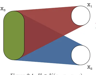
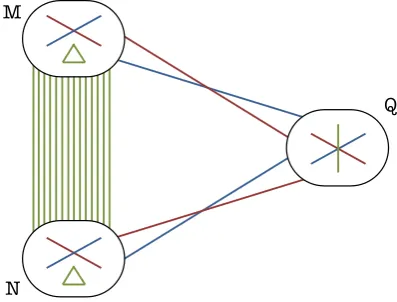
Definition 2.5.2. For x1, x2, x3, c positive, let K(x1, x2, x3, c) be the class of

edge-multicoloured graphs defined as follows:

A given three-multicoloured graphH = (V, E) belongs toK if its vertex set can be parti-tioned intoX1∪X2∪X3 such that

(i) |X1| ≥x1,|X2| ≥x2,|X3| ≥x3;

(ii) H is c-almost-complete;

(iii) (a) all edges present in H[X1, X3]are red,

(b) all edges present inH[X2, X3] are blue,

(40)

X₁

X2

[image:40.595.210.410.80.237.2]

X3

Figure 2.4: H_∈K(x1, x2, x3, c).

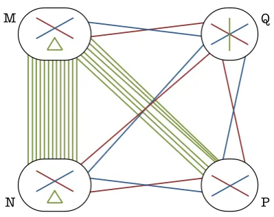
Definition 2.5.3. Forx1, x2, y1, y2, z, cpositive, letK∗(x1, x2, y1, y2, z, c) be the class of

edge-multicoloured graphs defined as follows:

A given three-multicoloured graph H = (V, E) belongs to _K∗, if its vertex set can be partitioned into X1∪X2∪Y1∪Y2 such that

(i) |X1| ≥x1,|X2| ≥x2,|Y1| ≥y2,|Y2| ≥y2,|Y1|+|Y2| ≥z;

(ii) H is c-almost-complete;

(iii) (a) all edges present in H[X1, Y1]and H[X2, Y2] are red,

(b) all edges present inH[X1, Y2] andH[X2, Y1] are blue,

(c) all edges present inH[X1, X2] andH[Y1, Y2] are green.

Y1 X₁

Y2 X2

Figure 2.5: H_∈K∗(x1, x2, y1, y2, c).

[image:40.595.207.400.481.652.2]

(41)

Theorem B. For everyα1, α2, α3>0 such thatα1≥α2, letting

c= max{2α1+α2,1₂α1+1₂α2+α3},

there exists ηB =ηB(α1, α2, α3) and kB =kB(α1, α2, α3, η) such that, for every k > kB

and every η such that 0< η < ηB, every three-multicolouring ofG, a (1−η4)-complete

graph on

(c−η)k≤K≤(c−1₂η)k

vertices, results in the graph containing at least one of the following:

(i) a red connected-matching on at least α1k vertices;

(ii) a blue connected-matching on at least α2k vertices;

(iii) a green odd connected-matching on at least α3k vertices;

(iv) two disjoint subgraphs H1, H2 from H1∪ H2, where

H1 =H

(α1−2η1/16)k,(1₂α2−2η1/16)k,3η4k, η1/16,red,blue

,

H2 =H

(α2−2η1/16)k,(1₂α1−2η1/16)k,3η4k, η1/16,blue,red

;

(v) a subgraph from

K(1₂α1−14000η1/2)k,(1₂α2−14000η1/2)k,(α3−68000η1/2)k,4η4k

;

(vi) a subgraph from _K∗₁_{∪ K}∗₂, where

K∗1 =K∗ (12α1−97η

1/2₎_k,₍1

2α1−97η

1/2₎_k,₍1

2α1+ 102η 1/2₎_k,

(1₂α1+ 102η1/2)k,(α3−10η1/2)k,4η4k,

K∗2 =K∗ (12α1−97η1/2)k,(12α2−97η1/2)k,(43α3−140η1/2)k,

100η1/2k,(α3−10η1/2)k,4η4k.

Furthermore,

(iv) occurs only if α3 ≤ 3₂α1+1₂α2+ 14η1/2 with H1, H2 ∈ H1 unless α2 ≥α1−η1/8;

(42)

This result forms a partially strengthened analogue of the main technical result of the paper of Figaj and Luczak [F L07b]. In that paper, Figaj and Luczak considered a similar graph but on slightly more than max{2α1+α2,1₂α1+ 1₂α2+α3}k vertices and proved

the existence of a connected-matching, whereas we consider a graph on slightly fewer vertices and prove the existence of either a monochromatic connected-matching or a particular structure.

2.6

Tools

In this section, we summarise results that we shall use later in our proofs beginning with some results on Hamiltonicity including Dirac’s Theorem, which gives us a minimum-degree condition for Hamiltonicity:

Theorem 2.6.1 (Dirac’s Theorem [Dir52]). If Gis a graph on n≥3 vertices such that every vertex has degree at least 1₂n, then G is Hamiltonian.

Observe then that, by Dirac’s Theorem, any c-almost-complete graph on n vertices is Hamiltonian, provided thatc_≤ 1₂n₋1. Then, since almost-completeness is a hereditary property, we may prove the following corollary:

Corollary 2.6.2. If G is a c-almost-complete graph on n vertices, then, for any inte-germ such that2c+ 2≤m≤n, Gcontains a cycle of length m.

Proof. Given G, a c-almost-complete graph on n vertices, let X ⊆ V(G) be such that |X| =m ≥2c+ 2. Then, G[X] is a c-almost-complete graph on |X| vertices so every vertex inG[X] has degree at least|X|−1−c= 1₂|X|+(1₂|X|−1−c)≥ 1

2|X|. Thus,G[X]

satisfies the conditions in Dirac’s Theorem and therefore contains a cycle on _|X_| =m

vertices. 2

Dirac’s Theorem may be used to assert the existence of Hamiltonian paths in a given graph as follows:

(43)

Proof. Given any two vertices x1, x2 ∈ V, let W = V\{x1, x2}. Then, G[W] has

n−2 vertices and has minimum degree at least 1₂(n−2) and so has a Hamiltonian cycle H. Since x1, x2 each have degree at least ₂1n to W, we can find u, v in W such

that ux1, vx2 ∈E and u, v are consecutive vertices in H. Thus, we can construct a

Hamiltonian path inGfrom x1 tox2. 2

For balanced bipartite graphs, we make use of the following result of Moon and Moser: Theorem 2.6.4 ([MM63]). If G = G[X, Y] is a simple bipartite graph on n vertices such that |X| = |Y| = 1₂n and d(x) +d(y) ≥ 1

2n+ 1 for every xy /∈ E(G), then G is

Hamiltonian.

Observe that, by the above, anyc-almost-complete balanced bipartite graph on n ver-tices is Hamiltonian, provided that c _≤ 1₄n₋ 1₂. Then, since almost-completeness is a hereditary property, we may prove the following corollary:

Corollary 2.6.5. If G = G[X, Y] is c-almost-complete bipartite graph, then, for any even integer m such that 4c+ 2 _≤ m _≤ 2 min_{|X_|,_|Y_|}, G contains a cycle on m vertices.

Proof. Given G=G[X, Y], a c-almost-complete bipartite graph, letU _⊆X,V _⊆Y be such that_|U_|=_|V_|= 1₂m_≥2c+1. Then,G[U, V] is ac-almost-complete bipartite graph so, for anyu _∈U and v _∈V, we have d(x) +d(y)_{≥ |}U_|+_|V_{| −}2c _≥ 1₂(_|U_|+_|V_|) + 1. Thus,G[U, V] satisfies the conditions for Theorem 2.6.4 and therefore contains a cycle

on_|U_|+_|V_|=mvertices. 2

For bipartite graphs which are not balanced, we make use of the Lemma below:

Lemma 2.6.6. IfG=G[X1, X2]is a simple bipartite graph onn≥4 vertices such that

|X1|>|X2|+ 1 and every vertex inX2 has degree at least 1₂n+ 1, then any two vertices

x1, x2 in X1 such that d(x2)≥2 are joined by a path which visits every vertex ofX2.

Proof. Observe that 1₂n+ 1 = 1₂_|X1|+1₂|X2|+ 1 =|X1| −(1₂|X1| −1₂|X2| −1) so any pair

of vertices inX2 have at least|X1| −(|X1| − |X2| −2) common neighbours and, thus, at

least_|X1| −(|X1| − |X2|)≥ |X2|common neighbours distinct fromx1, x2.

Then, ordering the vertices ofX2 such that the first vertex is a neighbour of x1 and the

(44)

For graphs with a few vertices of small degree, we make use of the following result of Chv´atal:

Theorem 2.6.7([Chv72]). IfGis a simple graph onn_≥3vertices with degree sequence d1 ≤d2≤ · · · ≤dn such that

dk≤k≤

n

2 =⇒ dn−k≥n−k,

thenG is Hamiltonian.

We also make extensive use of the theorem of Erd˝os and Gallai:

Theorem 2.6.8 ([EG59]). Any graph onK vertices with at least 1₂(m₋1)(K₋1) + 1

edges, where 3_≤m_≤K, contains a cycle of length at leastm.

Observing that a cycle onm vertices contains a connected-matching on at least m₋1 vertices, the following is an immediate consequence of the above.

Corollary 2.6.9. For any graph G on K vertices and any m such that 3 _≤ m _≤ K, if the average degree d(G) is at least m, then G contains a connected-matching on at least m vertices.

The following decomposition lemma of Figaj and Luczak [F L07b] also follows from the theorem of