Essays on Spatial Autoregressive
Models with Increasingly Many
Parameters
Abhimanyu Gupta
A thesis submitted to the Department of Economics of the
London School of Economics and Political Science for the degree
of Doctor of Philosophy
Declaration
I certify that the thesis I have presented for examination for the PhD degree of the London School of Economics and Political Science is solely my own work other than where I have clearly indicated that it is the work of others (in which case the extent of any work carried out jointly by me and any other person is clearly identified in it).
The copyright of this thesis rests with the author. Quotation from it is permitted, provided that full acknowledgement is made. This thesis may not be reproduced without my prior written consent.
I warrant that this authorisation does not, to the best of my belief, infringe the rights of any third party.
I declare that my thesis consists of 65,045 words.
Abstract
Much cross-sectional data in econometrics is blighted by dependence across units. A solution to this problem is the use of spatial models that allow for an explicit form of dependence across space. This thesis studies problems related to spatial models with increasingly many parameters. A large proportion of the thesis concentrates on Spatial Autoregressive (SAR) models with increasing dimension. Such models are frequently used to model spatial correlation, especially in settings where the data are irregularly spaced.
Chapter 1 provides an introduction and background material for the thesis. Chap-ter 2 develops consistency and asymptotic normality of least squares and instrumental variables (IV) estimates for the parameters of a higher-order spatial autoregressive (SAR) model with regressors. The order of the SAR model and the number of re-gressors are allowed to approach infinity with sample size, and the permissible rate of growth of the dimension of the parameter space relative to sample size is studied.
An alternative to least squares or IV is to use the Gaussian pseudo maximum likelihood estimate (PMLE), studied in Chapter 3. However, this is plagued by finite-sample problems due to the implicit definition of the estimate, these being exacerbated by the increasing dimension of the parameter space. A computationally simple Newton-type step is used to obtain estimates with the same asymptotic properties as those of the PMLE.
Chapters 4 and 5 of the thesis deal with spatial models on an equally spaced, d
-dimensional lattice. We study the covariance structure of stationary random fields defined on d-dimensional lattices in detail and use the analysis to extend many
Acknowledgements
I am greatly indebted to my supervisor, Professor Peter Robinson, for his invaluable support and guidance.
The econometrics faculty at LSE were extremely supportive and helpful. I am grateful to Javier Hidalgo, Tatiana Komarova, Oliver Linton, Taisuke Otsu, Marcia Schafgans and Myung Hwan Seo for all the help and feedback over the years
I would also like to thank fellow researchers at the LSE, in particular the partic-ipants at the work in progress seminars, for valuable feedback on my work. I had many enjoyable discussions with Abhisek Banerjee, Svetlana Bryzgalova, Ziad Daoud, Jungyoon Lee, Francesca Rossi and Sorawoot Tang Srisuma. Sometimes we actually talked about econometrics.
Outside of the econometrics group, particular thanks are due to my long-suffering office-mates Wenya Cheng and Attakrit Leckcivilize, who stoically accepted the pres-ence of a theoretical econometrician in their midst. Kitjawat Tacharoen, Daniel Ver-nazza and Mazhar Waseem ensured that there were always lighter moments.
Contents
Contents 6
List of Tables 8
List of Figures 9
1 Introduction 10
1.1 Issues in the analysis of spatial data . . . 10
1.2 Spatial autoregressions for irregularly-spaced data . . . 11
1.3 Spatial autoregressions for regularly-spaced lattice data . . . 15
1.4 Increasingly many parameters . . . 18
1.5 Contributions of this thesis . . . 20
1.6 Some notation and definitions . . . 21
2 IV and OLS estimation of higher-order SAR models 23 2.1 Introduction . . . 23
2.2 Model and basic assumptions . . . 23
2.3 Consistency and asymptotic normality . . . 25
2.3.1 IV estimation . . . 25
2.3.2 Least squares estimation . . . 30
2.4 Applications . . . 33
2.4.1 Farmer-district type models . . . 33
2.4.2 Panel data SAR models with fixed effects . . . 33
2.4.3 Another illustration . . . 35
2.5 Empirical example: A spatial approach to estimating contagion . . . 36
2.A Matrix norm inequalities and notation . . . 42
2.B Proofs of results in Section 2.3 . . . 42
2.C Technical lemmas . . . 54
2.D Proofs of sundry claims . . . 55
3 Pseudo maximum likelihood estimation of higher-order SAR models 57 3.1 Introduction . . . 57
3.2 Pseudo ML estimation of Higher-Order SAR Models . . . 58
3.2.1 Mixed-Regressive SAR Models . . . 58
3.2.2 Pure SAR Models . . . 62
3.3 Finite-sample performance of PMLE . . . 63
3.4 Approximations to Gaussian PMLE . . . 68
4 Results for covariances of autoregressive random fields defined on
regularly-spaced lattices 108
4.1 Introduction . . . 108
4.2 Bounds for w-th absolute moments of partial sums, w∈(1,2] . . . 109
4.3 Covariance structure of stationary lattice processes with autoregressive half-plane representation . . . 111
4.3.1 d=2 . . . 112
4.3.2 d=3 . . . 114
4.3.3 Generald . . . 118
4.4 Counting covariances in stationary and unilateral lattice autoregressive models . . . 122
4.A Proof of Lemma 4.1 . . . 125
5 Consistent autoregressive spectral density estimation for stationary lattice processes 127 5.1 Introduction . . . 127
5.2 Truncated approximation of unilateral autoregressive processes . . . 129
5.3 Preliminary results on covariances and covariance estimates . . . 131
5.4 Uniform consistency of ˆfp(λ) . . . 134
5.A Proofs of theorems . . . 137
5.B Proofs of lemmas . . . 141
References 146
List of Tables
2.1 Summary of estimates of coefficients corresponding to weighting
matri-ces in specification (2.5.1) . . . 38
2.2 Summary of estimates of coefficients corresponding to weighting matri-ces in specification (2.5.2) . . . 39
2.3 List of countries and region classification for Section 2.5 . . . 41
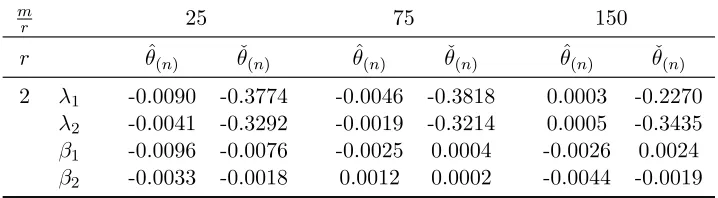
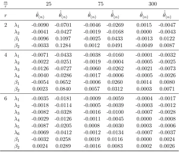
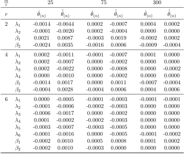
3.1 Monte Carlo Mean and Bias of ML Estimates . . . 64
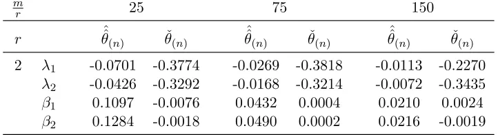
3.2 Monte Carlo Bias of IV and ML estimates . . . 64
3.3 Monte Carlo Relative MSE of IV and ML estimates . . . 65
3.4 Monte Carlo Relative Variance of IV and ML estimates . . . 65
3.5 Monte Carlo Bias of IV and Newton-step estimates, Xn∼U(0,1) . . . . 76
3.6 Monte Carlo Bias of IV and Newton-step estimates, Xn∼U(0,5) . . . . 77
3.7 Monte Carlo Relative MSE of IV and one-step estimates, Xn∼U(0,1) . 79 3.8 Monte Carlo Relative MSE of IV and one-step estimates, Xn∼U(0,5) . 80 3.9 Monte Carlo Relative Variance of IV and one-step estimates,Xn∼U(0,1) 81 3.10 Monte Carlo Relative Variance of IV and one-step estimates,Xn∼U(0,5) 82 3.11 Monte Carlo Bias of one-step and ML estimates, Xn∼U(0,1) . . . 83
List of Figures
1.1 Half-plane and quarter-plane representations of two-dimensional lattice
processes . . . 16
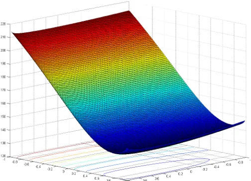
3.1 Sample Log-Likelihood Surface, r= 2, m= 50 . . . 66
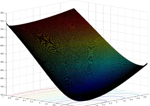
3.2 Sample Log-Likelihood Surface, r= 2, m= 150 . . . 67
3.3 Sample Log-Likelihood Surface, r= 2, m= 300 . . . 67
1
Introduction
In this chapter we provide the necessary background to evaluate the contribution of this thesis to the spatial econometrics and spatial statistics literature. Section 1.1 summarizes the key properties of spatial data and discusses solutions for issues that arise in the analysis of such data. Section 1.2 introduces spatial autoregressions for irspaced data, while Section 1.3 does the same for data on a regularly-spaced lattice. These sections also provide motivation for the analysis of higher-order autoregressions. Section 1.4 summarizes the literature on models with increasingly many parameters, while Section 1.5 outlines the contribution of this thesis to the literature. Finally, Section 1.6 introduces some notation and definitions that will be used throughout the thesis.
1.1 Issues in the analysis of spatial data
Correlation in cross-sectional data poses considerable challenges to econometricians and statisticians, complicating both modelling and statistical inference. In economet-rics, a substantial literature collectively known as Spatial Econometrics has analysed the problems caused by correlation between observations at different points in space. This goes back as far as the early work by Moran (1950), and key waypoints in the journey of the literature have been the contributions by Cliff and Ord (1973) and Cressie (1993). Survey articles outlining recent developments in spatial econometrics include Robinson (2008) and Anselin (2010). A feature of the spatial econometrics literature is its focus on spatial data recorded at irregularly-spaced points. This is reflective of typical datasets available in economic applications. Due to the irregu-larity of the spacing and the ambiguity about the process generating the locations of observations, fairly strong assumptions are necessary to capture spatial correlation parsimoniously. In this thesis, we will concentrate on a class of assumptions that give rise to an ‘autoregressive’ model.
On the other hand, much of the spatial statistics literature has focused on data recorded on a regularly-spaced d-dimensional lattice, where d > 1. Typically the
the original multilateral model, as the coefficients in the unilateral representation may not have a closed-form expression in terms of the original ones even with seemingly simple multilateral models. However, as we show in Chapters 4 and 5, such unilateral representations can be extremely useful if our interest lies in prediction and spectral density estimation. Another complication is the bias in covariance estimates due to the ‘edge-effect’, noted by Guyon (1982) who proposed an incorrectly centred version of the covariance estimates to eliminate this effect. The edge-effect worsens with increas-ing d. Solutions to the edge-effect are also explored in Dahlhaus and K¨unsch (1987)
and Robinson and Vidal Sanz (2006).
1.2 Spatial autoregressions for irregularly-spaced data
The reader may wonder if the theory of irregularly-spaced time series can be extended to the case of irregularly-spaced spatial data, just as we discussed the extension of the theory of regularly-spaced time series to many dimensions above. Robinson (1977) showed that some cases of irregularly-spaced time series can be described by an un-derlying continuous time process where spacing is generated by a point process. When the continuous time process is a first-order stochastic differential equation with con-stant coefficients and driven by white noise, consistent and asymptotically normal estimates of the unknown parameters can be obtained from an approximated Gaus-sian log-likelihood. This can be extended to situations when the data are recorded at irregularly-spaced geographical locations, but even then leads to complications in estimation and inference.
Besides such complications, ‘space’ in economic applications need not refer to geo-graphic space. In fact the notion of economic distance encompasses many more possi-bilities (e.g. differences in income of economic agents), of which geographic distance is but one, and this notion of distance determines the spatial correlation between obser-vations. In spatial econometrics, the economic distance between two economic agents (also called units)iandjis defined as the distance between two vectors of
characteris-ticsvi andvj. Note that we identified units with their location. This distance may be
defined in a number of ways, without any geographical interpretation (see e.g. Conley and Ligon (2002), Conley and Dupor (2003)). If there is no geographical interpretation of the distance, any hope of extending the theory of irregularly-spaced time series is extinguished.
Instead, a commonly used framework for describing such data is the spatial autore-gressive model, introduced by Cliff and Ord (1973, 1981). Given a sample of sizen, the
problem of irregular-spacing and location is circumvented by the introduction of an
n×nspatial weights matrix, denoted Wn, which is chosen by the practitioner
wij,nofWnare inversely related to some measure of economic distance. This distance
need not be geographic distance, as discussed above. The wij,n may be binary, for
instance taking the value 1 when two units are contiguous according to some definition of contiguity, and 0 otherwise. The SAR model can also be combined with explanatory variables to give rise to the mixed regressive SAR (MRSAR) specification, and multiple weight matrices may be included to cover spatial correlation arising from a variety of sources or from higher orders of spatial contiguity. A caveat is that adding more weight matrices can lead to circularity in dependence (see Blommestein (1985)), so care must be taken to guard against such redundancies to avoid identification problems.
For an n×1 vector of observationsyn, ann×k matrix of regressors Xnand n×n
weight matrices Win, i= 1, . . . , p, it is assumed that there exist scalars λ1, λ2, . . . , λp
and ak×1 vector β such that
yn= p X
i=1
λiWinyn+Xnβ+Un (1.2.1)
whereUnis ann×1 vector of disturbances. In this thesis we will refer to the MRSAR
model as simply SAR and the SAR model without regressors as the pure SAR. Typically diagonal elements of Wn are normalised to zero (see Assumption 2 and
its discussion below). Another normalisation that weight matrices are frequently sub-jected to is row-normalisation, which ensures that each row of the normalised Win
sums to 1. In this case, taking p= 1 for illustrative purposes, the (i, j)-th element of W1n is
wij,n=
dij,n Pn
h=1dih,n
(1.2.2)
where dij,n is some measure of distance between observations at locations i and j.
This provides motivation for allowing the wij,n to depend on n, even if the dij,n do
not, implying that the yn should be treated as triangular arrays as reflected in the
subscripting with n. Kelejian and Prucha (2010) observed that if the weight matrices
are subjected to a normalisation that is a function of sample size, the autoregressive parameters corresponding to the normalised weight matrices in the transformed model are dependent onneven if the original ones were not. It is clear that row-normalisation
is an example of such a normalisation. The regressor matrix Xn may also contain
spatial lags, and so it is attractive to allow both the autoregressive and regression parameters to vary with n. It is possible that dij,n6=dji,n so that spatial interactions
are allowed to be asymmetric. See e.g. Arbia (2006) for a recent review of spatial autoregressions.
gen-erally presented forp= 1 i.e. the model
yn=λWnyn+Xnβ+Un. (1.2.3)
The presence of spatially lagged yn on the right side causes endogeneity problems,
leading to ordinary least squares (OLS) estimation being summarily dismissed in much of the early spatial econometrics literature. However Lee (2002) showed that under additional conditions on thewij,nOLS estimation can be consistent and asymptotically
efficient. In particular, lethn be a sequence that is bounded away from zero uniformly
inn, and let primes indicate transposition. Lee (2002) proved that the OLS estimate
of (λ, β0)0 in (1.2.3) is consistent if hn→ ∞and thewij,nare defined as in (1.2.2) with
thedij,nsatisfying
c < Pn
h=1dih,n hn
,
where c is a generic, arbitrarily small but positive constant that is independent of n.
If additionallyn12/hn→0 asn→ ∞, then the OLS estimates are also asymptotically
normal.
The instrumental variables (IV) estimate of Kelejian and Prucha (1998) is n12
-consistent (and also applicable to a version of (1.2.1) that allows for spatially corre-lated disturbances) under less restrictive conditions than the least squares estimate, since the introduction of hn is not required, but is not efficient. On the other hand,
it is computationally simpler than the generalized method of moments (GMM) esti-mate of Kelejian and Prucha (1999) and the (Gaussian) pseudo maximum likelihood estimate (PMLE) studied by Lee (2004), these being implicitly defined. The latter is obtained by maximising a Gaussian likelihood even when the disturbances are not actually Gaussian. If Gaussianity obtains, then the PMLE becomes the Maximum Likelihood Estimate (MLE) and is efficient in the Cram´er-Rao sense. In fact, the asymptotic variance of the OLS estimates coincides with that of the MLE. Robinson (2010) developed asymptotic theory for efficient estimation of a semiparametric version of (1.2.1). Lee (2003) has also provided the optimal instruments for the IV estimator of Kelejian and Prucha (1998). For general, but fixed p, Lee and Liu (2010) justify an
efficient GMM estimate.
The regressorsXnplay a key role in estimation, with IV and OLS estimation
possi-ble only in their presence. The presence of even one non-intercept regressor can identify the spatial component of the model, as the regressor creates the correct deflation in the OLS and IV estimates. Without this deflation the deviation of the estimate from the true value converges to a non-degenerate distribution. As a result, the pure SAR model
yn= p X
i=1
cannot be estimated using a closed-form estimate in general. One implication of this observation is that IV and OLS estimates cannot be used to test the null hypothesis
β= 0 in (1.2.1).
In Chapters 2 and 3, the spatial lag order pin (1.2.1) and the number of regressors kare allowed to increase slowly with n, as opposed to being fixed. This has attractions
in that it allows for a richer model with increasing data. However, we now demonstrate by means of an example that such an asymptotic regime can arise quite naturally from applications.
A specification for the weight matrix that is frequently used for illustrative and simulation purposes is that used in Case (1991, 1992). In her scenario data are recorded inr districts, each of which contains m farmers, implying n=mr. It is assumed that
farmers within each district impact each other equally and that there is inter-district independence between farmers so that we have
Win =diag
0, . . . , |{z}Bm ithdiagonal block
, . . . ,0
. (1.2.4)
with
Bm= 1
m−1 lml
0
m−Im (1.2.5)
where lm is the m-dimensional vector of ones (1, . . . ,1)0 and Im the m-dimensional
identity matrix.
With such a natural partitioning of the data, it is likely that the SAR parameters are unequal across districts. The true values may vary according to the properties of districts e.g. geographic or demographic differences to mention just two. Consider the model
yn= r X
i=1
λiWinyn+Xnβ+Un, (1.2.6)
contrasted with currently available theory, discussed above, that typically considers the specification (1.2.1) withp= 1 and
Wn=diag[Bm, . . . , Bm]. (1.2.7)
If we allow n → ∞ with both m → ∞ and r → ∞ then the number of λis increase
withn at rate r so that it is quite natural to consider an ‘increasing-order’ version of
(1.2.1) wherep→ ∞ asn→ ∞. In fact, as we demonstrate in Chapter 2, applications
may even imply that both p → ∞ and k → ∞ as n→ ∞. As a result we introduce
1.3 Spatial autoregressions for regularly-spaced lattice data
As mentioned before, the extension of time-series theory to even regularly-spaced lat-tices is not straightforward. We present a summary of the problems using examples from Whittle (1954). We first illustrate dependence from many directions by means of a simple bilateral model in one dimension (d = 1), and demonstrate that this can
be converted into a unilateral model. Denoting observations by xt and errors by t, a
simple bilateral autoregression in one dimension is
xt=αxt−1+βxt+1+t. (1.3.1)
The estimation of this model by minimizing over α and β the usual least squares
objective function
U(α, β) =X t
(xt−αxt−1−βxt+1)2
leads to nonsensical results. This is due to the omission of the Jacobean of the trans-formation from t toxt, which is not unity for (1.3.1). The correct objective function
is in fact k(α, β)U(α, β) with
logk(α, β) =− 1
2π Z 2π
0
log αeıω−1 +βe−ıω αe−ıω−1 +βeıωdω.
Evaluating the integral yields the objective function
n
1 + (1−4αβ)12
o−2X
t
(xt−αxt−1−βxt+1)2. (1.3.2)
In fact (1.3.1) can be given a unilateral representation which generates the same au-tocorrelation function. Let aand b−1 be the roots of the polynomial α−z+βz2 and
defineA and B by comparing coefficients in
(z−a)(z−b) =z2+Az+B. (1.3.3)
Then the AR(2) process
xt+Axt−1+Bxt−2 =t
generates the same autocorrelations as (1.3.1). Transformation to A and B reveals
that (1.3.2) is proportional to
X
t
(xt+Axt−1+Bxt+1)2.
(1.3.3).
In contrast, matters are substantially more complicated in two dimensions. To illustrate this we first explain what is meant by a unilateral model in two dimensions. Suppose thatxst is an observable variate with each subscript being integral and
denot-ing location in the respective dimension, andst be the unobservable error. We call an
autoregression of the variate xst unilateral if it can be expressed as an autoregression
of xst on xsu and xvw withu > t, v > sand w unrestricted (also see Wiener (1949)).
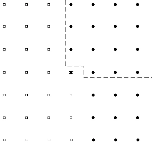
In the lattice of Figure 1.1, this means that the observation at the cross be must ex-pressible in terms of of the observations at the black dots. The diagram motivates the use of the term ‘half-plane’. Such a representation ensures a Jacobean that does not depend on the parameters, and implies that the parameters of the unilateral scheme are estimable by least-squares. The idea is easily extended to d >2. We also illustrate
the case of ‘quarter-plane’ dependence, a special case of half-plane dependence, by the region bounded by the dashed lines.
[image:16.595.186.435.402.641.2]The definition of a half-plane or quarter-plane is clearly not unique but we will adopt the description of the previous paragraph and Figure 1.1 as convention (without loss of generality) in this thesis.
Figure 1.1: Half-plane and quarter-plane representations of two-dimensional lattice processes
impossible. The seemingly straightforward bilateral, d= 2 model
xst =α(xs+1,t+xs−1,t+xs,t+1+xs,t−1) +st
has a unilateral representation with coefficients that are expressible in no simpler form than elliptical integrals, hence yielding no closed-form. Matters are complicated further because unilateral representations of finite autoregressions may be infinite. Indeed, the finite autoregression
(1 +β2)xst =β(xs+1,t+xs,t+1+xs,t−1) +st
has an infinite unilateral representation given by
xst = 2βxs,t+1−β2xs,t+2−β2xs+1,t+1+β 1−β2
X∞
j=0
βjxs+1,t−j+0st, (1.3.4)
where 0st is a white noise error term. Whittle (1954) proposes an approximation to
the Gaussian likelihood, now called the Whittle likelihood, that permits estimation of the parameters in multilateral models.
On the other hand, the unilateral representation is extremely useful if our interest is in prediction purposes, or in spectral density estimation. The spectral density of the process xst may estimated through least-squares estimation of the unilateral
autore-gressive representation. Autoreautore-gressive spectral estimation is well-established in time series, with roots in the contribution of Mann and Wald (1943). The advantages of autoregressive spectral estimation for time series were listed in Parzen (1969). These are enumerated in Chapter 5. The work of Akaike (1969) and Kromer (1970) estab-lished the techniques for this approach to estimating the spectrum with time series data. For spatial processes, this has been studied in a vast signal processing litera-ture. Tjøstheim (1981) considers an autoregression defined unilaterally on a quarter plane and finds some evidence that autoregressive spectral estimation is superior to conventional spectral analysis methods. McClellan (1982) reviews seven different types of spectral estimates, the autoregressive estimator being one of them. Wester, Tum-mala, and Therrien (1990) propose iterative techniques to optimise computation of autoregressive estimates in both the half-plane and quarter-plane case.
such as (1.3.4). While it may be argued that truncated versions of (1.3.4) such as
xst= 2βxs,t+1−β2xs,t+2−β2xs+1,t+1+β 1−β2
k X
j=0
βjxs+1,t−j+0st
need to be employed in practice, it is desirable to letk → ∞as the sample size increases
to overcome the bias caused by using a finite autoregression. Even for time series, finite autoregressions may not capture the data generating process (DGP) and, for the regularly-spaced time series case, Berk (1974) provides results on the consistency and asymptotic normality of spectral density estimates with the order of the autoregression allowed to diverge with sample size. This approach has added appeal because any stationary, purely non-deterministic (in the linear prediction sense) time series has an infinite moving-average representation which, under invertibility conditions, yields an infinite autoregressive representation.
In Chapters 4 and 5, we extend Berk’s consistency result to lattice processes. While we have already discussed that any multilateral process has a (possibly infinite) unilateral representation, Helson and Lowdenslager (1958, 1961) showed that even more generally all stationary, purely non-deterministic (in the linear prediction sense) spatial processes have a half-plane, infinite, moving-average representation. Again under invertibility conditions we can use this to write down an infinite autoregressive half-plane representation that is estimable by least-squares. As a result, there is strong motivation for an extension of the result of Berk (1974). We have seen that even for processes that already have a multilateral representation, the corresponding unilateral scheme may be infinite. This provides even greater reason to study the estimation of unilateral spatial autoregressions with diverging order in all dimensions. Extension is not straightforward, with complications arising due to the structure of the covariance matrix and the edge-effect.
1.4 Increasingly many parameters
considers the multiple regression model
y=Xβ+ (1.4.1)
when the dimension ofβ is allowed to diverge with sample size. Let xi denote thei-th
column of X0 and yi the i-th element of the n-dimensional vector y. The M-estimate
ofβ, denotedβM, is the vector that solves
n X
i=1
xiψ yi−x0iβ
= 0,
where ψ:R →R is a given function. The least squares estimate is a particular case
with ψ(x) = x. The asymptotic properties of βM are then studied. This problem is
considered further in Yohai and Maronna (1979) and Ringland (1983). The former showed that if the dimension of β is p, withp→ ∞, thenp2/n→0 is sufficient for
kβM −βk−→p 0, (1.4.2)
where we employ Euclidean norm (see Section 1.6), and p52/n→0 is sufficient for
a0(βM −β)−→d N(0,1), (1.4.3)
where ais some appropriately bounded vector in Rp. Portnoy (1984, 1985) improves
the conditions for (1.4.2) and (1.4.3) to plogp/n→0 and (plogp)32 /n respectively.
We have already mentioned the contribution of Berk (1974) to the time series increasing parameter literature. He proves that for an autoregression of order k with k→ ∞ asn→ ∞, least-squares estimates of autoregression coefficients are consistent
and asymptotically normal in the sense of (1.4.2) and (1.4.3) if k2/n → 0 and the
resulting spectral density estimate is consistent and asymptotically normal if k3/n→
0. Robinson (1979) establishes similar conditions for truncated approximations to systems with infinite distributed lags, but allows these conditions to vary with the strength of the assumptions on existence of moments for the errors. In Robinson (2003) simultaneous equation models with increasingly many equations are considered, which is equivalent to studying increasingly many coefficients on the endogenous and exogenous variables. It is shown that if the number of exogenous variables, m, is
allowed to increase with n, then m2/n → 0 is sufficient for asymptotic normality of
instrumental variable (IV) estimates of the parameters of a single equation nested in a system with increasingly many equations.
mentioned that for such models Moreira (2009) has suggested a method based on using group actions and invariants (see also Eaton (1989)) to construct an objective function that is a function of a parameter of fixed dimension. The disadvantage of this approach is that the incidental parameters are treated purely as nuisance parameters and not actually estimated. In contexts such as the setting of Case (1991, 1992) discussed in Section 1.2, the incidental parameters are actually of interest and indeed tests of equality between them can be extremely useful in applied work.
1.5 Contributions of this thesis
This thesis makes several contributions. We list these by chapter. In Chapter 2, con-sistency and asymptotic normality of IV and OLS estimates in a SAR model with increasing autoregressive order and increasingly many regressors is considered. Per-missible rates of growth of the parameter space relative to sample size are derived. This is more complicated than the model (1.4.1), due to the presence of spatially lagged
yn. In addition an empirical example illustrates a prescription for applied work: if the
model design implies heterogeneity in spatial units then the spatial parameters should also reflect this.
Chapter 3 studies pseudo maximum likelihood estimates for the model considered in Chapter 2. The problem is challenging as it involves an implicitly defined estimate of a parameter of increasing dimension. A Monte Carlo study reveals that even the MLE suffers from finite-sample identification problems. Motivated by this, we also propose closed-form estimates obtained from a Newton-type step commencing from the IV and OLS estimates of Chapter 2. These are shown to have the same asymptotic distribution as the PMLE and their finite-sample properties are studied in a Monte Carlo experiment.
Chapters 4 and 5 concentrate on autoregressions defined on a regularly-spaced d
-dimensional lattice. In particularly we focus on half-plane representations, which can be estimated by least-squares. Unlike in the time-series, unilateral representations of stationary processes do not yield a Toeplitz covariance matrix. Chapter 4 demonstrates that for spatial processes the covariance matrix may be nested inside a matrix which is block-Toeplitz with Toeplitz-blocks with d−1 levels of nesting. This contribution is
spatial processes.
In Chapter 5 of this thesis, we exploit the structure derived in Chapter 4 to propose an autoregressive spectral density estimate for a stationary lattice process and prove that this is uniformly consistent under conditions that restrict the rate of growth of the autoregressive order in all dimensions. This is an important result due to the advantages of autoregressive spectral estimation listed in Section 1.3, and also because of the problems caused by the edge-effect in kernel-based spectral density estimation.
1.6 Some notation and definitions
We introduce some notation and definitions. These will be used throughout the thesis.
1. 1(∙) denotes the indicator function i.e.
1(x∈A) = (
1 ifx∈A;
0 ifx /∈A.
2. For a generic p ×p matrix A with real eigenvalues, the largest and smallest
eigenvalues are denoted η(A) andη(A) respectively.
3. k∙kdenotes spectral norm i.e. for a generic real p×q matrix B,
kBk=η(B0B) 12 .
For vectors b we define Euclidean norm as (b0b)12, so that spectral norm and
Euclidean norm coincide for vectors.
4. For a generic realp×q matrixB = [bij] we define
kBkR= maxi=1,...,p q X
j=1
|bij|
and
kBkC = maxj=1,...,q p X
i=1
|bij|,
which are the maximum absolute row-sum and column-sum norms respectively. If someWinis row-normalized as in Section 1.2, then this implies that kWinkR= 1
if also Win has non-negative elements.
5. k∙kF denotes the Frobenius norm i.e. i.e. for a generic real p×q matrixB
kBkF =
p X
i=1
q X
j=1
b2ij
1 2
6. Throughout the thesis,Cwill denote a generic, arbitrarily large and positive
con-stant that is independent of sample size, whilecwill denote a generic, arbitrarily
small and positive constant that is independent of sample size.
7. Consistency: In this thesis, consistency of a parameter of increasing dimension is taken to mean consistency in Euclidean norm i.e. by the statement “θe is a
consistent estimate of θ” we mean
kθe−θk−→p 0.
Similarly, if we say that a matrix B of increasing dimensions can be consistently
estimated byBe we mean that
2
IV and OLS estimation of
higher-order SAR models
2.1 Introduction
In this chapter a version of (1.2.1) is considered wherep, k → ∞asn→ ∞. This allows
for more flexible modelling, in accordance with the idea that more parameters may be estimated as we increase the sample size, and explicitly permits asymptotic regimes prevalent in applied situations, as we illustrate later. Increasingly many parameters have been extensively studied in multiple regression, for instance by Huber (1973) and in a series of papers by Portnoy (1984, 1985). Berk (1974) and Robinson (2003) also studied problems with increasingly many parameters in time series autoregressions and simultaneous equations systems respectively. This literature has been discussed in Chapter 1.
In the next section, we introduce and discuss our model and also introduce some ba-sic assumptions. Conditions and theorems for the consistency and asymptotic normal-ity of least squares and instrumental variable (IV) estimates are presented in Section 2.3. In Section 2.4, we consider applications while Section 2.5 provides an empirical example. The proofs of the theorems and the sequences of lemmas that they rely on are left to appendices.
2.2 Model and basic assumptions
Given the existence of vectors λ(n) = (λ1n, . . . , λpnn)0 and β(n) = (β1n, . . . , βknn)
0,
where 0 indicates transposition, we wish to model the n×1 observable vector y
n =
(y1n, . . . , ynn)0 by the specification
yn= pn
X
i=1
λinWinyn+Xnβ(n)+Un (2.2.1)
withpn→ ∞ asn→ ∞,Xn an n×kn matrix of constants with kn→ ∞ asn→ ∞
and Un= (u1, . . . , un)0 a vector of unobservable disturbances. We may rewrite (2.2.1)
as
Snyn=Xnβ(n)+Un (2.2.2)
whereSn =In−Ppi=1n λinWin or equivalently yn=Rnλ(n)+Xnβ(n)+Un with Rn=
(W1nyn, . . . , Wpnnyn). Note that in contrast to (1.2.1), in (2.2.1) we also allow the individual λ(n) and β(n) elements to vary withn as discussed in the previous section.
model. Although Portnoy (1984, 1985) allowed his model to have stochastic regressors, these were not generated using a spatial process. In fact, in some sufficient conditions they were taken to be i.i.d.
Recently there has also been some interest in the estimation of spatial weight matri-ces, as opposed to assuming that they are exogenously chosen, see e.g. Bhattacharjee and Jensen-Butler (2013). A potential extension of the model considered in this chap-ter is to spatial weight matrix estimation, where each unit is influenced by a number of neighbours that increases slowly with sample size. In this case the quantities of interest are the elements of the weight matrices themselves, but these may be treated as linearly occurring parameters using suitable decompositions of the weight matrix/matrices, or a partitioning of the spatial domain.
We now introduce some basic assumptions.
Assumption 1. Un= (u1, . . . , un)0 has iid elements with zero mean and finite variance σ2.
Assumption 2. Fori = 1, . . . , pn, the elements of Win are uniformly O(1/hn), where hn is some positive sequence which may be bounded or divergent. If it is bounded,
then it must also be bounded away from 0. The diagonal elements of each Win are
zero. We additionally assume thatn/hn→ ∞ asn→ ∞.
Different hin sequences for each of theWinmay be used. However for least squares
estimation, even for fixed p, Lee (2002) demonstrated that consistency requires
diver-gence so that mini=1,...,pnhin→ ∞ must be assumed and Assumption 2 entails no loss of generality. He also provides a detailed discussion of this assumption. In IV estima-tion, any mixture of bounded and divergenthin sequences may be employed. However
boundedness away from zero is crucial as even consistency of the error variance esti-mate based on IV residuals may fail if this does not hold. Indeed, an interpretation of
hn is that it is the number of neighbours of a unit and it is rather odd to allow this to
go to zero as the sample size increases. The diagonal elements being zero implies that a unit is not regarded as its own neighbour.
Assumption 3. Sn is non-singular for sufficiently large n.
This assumption ensures that (2.2.2) has a solution for yn. If the Win happen to
be block diagonal with a single non-zero block such that kWinkR≤1 fori= 1, . . . , d,
then we prove in Appendix 2.D that a sufficient condition for Sn to be non-singular is
Assumption 4. Sn−1R, Sn−1C, kWinkR and kWinkC are uniformly bounded in n
and ifor all i= 1, . . . , pn and sufficiently largen.
This assumption has its provenance in Kelejian and Prucha (1998). The parts pertaining to S−1
n ensure that the spatial correlation is curtailed to a manageable
degree because the covariance matrix ofynisσ2Sn−1Sn0−1. The assumptions on theWin
are satisfied trivially if one unit is assumed to be a ‘neighbour’ of only a finite number of other units, and is also satisfied if a unit is a neighbour of infinitely many units as long as the wij,n decline fast enough. The latter is natural if the wij,n are decreasing
functions of some measure of distance between units.
Assumption 5. The elements ofXn are constants and are uniformly bounded in n, in
absolute value, for all sufficiently large n.
The assumption of non-stochastic regressors has been fairly standard in the the-oretical spatial econometrics literature dealing with OLS estimation and the PMLE, see e.g. Lee (2002) and Lee (2004). In Kelejian and Prucha (1999) all expectations are to be read as conditional on the realisations of the explanatory variables, and so the regressors are treated as fixed in their theory. Assumption 5 is certainly strong, but we opt for it as the main purpose of this chapter is to study the implications of the increasing order of the SAR model. A similar discussion applies to Assumption 6 in the next section.
2.3 Consistency and asymptotic normality
2.3.1 IV estimation
Because of the endogeneity of the Winyn, i = 1, . . . , pn, IV estimation has been
em-ployed for estimation of SAR models. LetZnbe ann×rn matrix of instruments, with rn≥pn for alln and introduce
Assumption6. The elements ofZnare constants and are uniformly bounded in absolute
value.
For the model (1.2.1) withp= 1, Kelejian and Prucha (1998) noted thatWnE(yn)
can be written as an infinite linear combination of the columns of the matrices
Xn, WnXn, Wn2Xn, . . . ,
assuming the existence of a convergent power (Neumann) series for (In−λWn)−1.
instrument matrix be constructed from linearly independent subsets of the columns of
Xn, WnXn, Wn2Xn, . . . , WnqXn,
where in principle q→ ∞ asn→ ∞but q = 2 was regarded as sufficient from Monte
Carlo experiments. Our theory allows the number of instruments to increase with sample size and provides a new result for the case when pnis fixed while rn is allowed
to diverge with n. For the specification (2.2.1), we will have
E(yn) = In− pn
X
i=1
λinWin !−1
Xnβ(n)
=
X∞
k=0
pn
X
i=1
λinWin !k
Xnβ(n), (2.3.1)
assuming that the power series is well-defined, so that instruments may be constructed as subsets of the linearly independent columns of
Xn, W1nXn, W12nXn, . . . , W2nXn, W22nXn, . . . , WpnnXn, W
2
pnnXn, . . . (2.3.2)
Columns ofXn pre-multiplied by cross-products of the Win may also be employed in
view of (2.3.1). Of course, other choices of instruments from outside the model are available to the practitioner depending on the problem under consideration.
We now provide sufficient conditions for the power series in (2.3.1) to be well-defined. A sufficient condition is
pn
X
i=1
λinWin
<1, (2.3.3)
for which either
max
i=1,...,pn;n≥1 |
λin| pn
X
i=1
Win
<1, (2.3.4)
or
max
i=1,...,pn;n≥1 k
Wink
Xpn
i=1
|λin|<1 (2.3.5)
suffices. When theWin take the form (1.2.4), thenPpi=1n Win=Wnas given in (1.2.7). Bm as defined in (1.2.5) has one eigenvalue equal to 1 and also −1/(m −1) as an
eigenvalue with multiplicity m−1. Hence kWnk=kWink=kBmk= 1, i= 1, . . . , pn,
and max
i=1,...,pn;n≥1 |
λin|<1 is sufficient for the power series to be valid, by (2.3.4). See
also Proposition 2.7 in Appendix 2.D for an equivalent result. The condition from (2.3.5) is much stronger in this setting, requiring that Ppn
Denoting θ(n)=λ0(n), β(0n), define the IV estimate of θ(n) as
ˆ
θ(n)= ˆQ−n1Kˆn0Jn−1ˆkn, (2.3.6)
with
ˆ
Qn= ˆKn0Jn−1Kˆn
where
ˆ
Kn= 1
n "
Zn0 Xn0
#
[Rn, Xn], knˆ = 1 n
" Zn0 Xn0
#
yn, Jn= 1 n
" Zn0 Xn0
#
[Zn, Xn].
This implies that
ˆ
θ(n)−θ(n)= ˆQn−1Kˆn0Jn−1qn,
where
qn= 1 n
" Zn0 Xn0
# Un.
Since (2.2.2) and Assumption 3 imply that yn = Sn−1Xnβ(n)+Sn−1Un we can write Rn=An+Bn where
An= (G1nXnβ(n), . . . , GpnnXnβ(n)), Bn= (G1nUn, . . . , GpnnUn),
and Gin =WinSn−1 fori= 1, . . . , pn. Also define
Kn=
1
n "
Zn0 Xn0
#
[An, Xn], Qn=Kn0Jn−1Kn, Ln=
1
n "
A0n Xn0
#
[An, Xn].
Note that Jn and Ln are symmetric matrices.
Introduce the following assumptions.
Assumption 7. lim
n→∞η(Jn)<∞ and limn→∞
η(Kn0Kn)>0.
Assumption 8. lim
n→∞
η(Jn)>0 and lim n→∞η(K
0
nKn)<∞.
These are asymptotic non-multicollinearity and finiteness conditions, which can to some extent be checked as we discuss in the next sub-section.
Lemma 2.1. Under Assumptions 7 and 8 respectively (i) lim
n→∞
η(Qn)>0.
(ii) lim
For just-identified (i.e. IV) estimation, we have pn=rn implying that ˆKn and Kn
are square matrices so that ˆθ(n)= ˆK−1
n ˆkn and Q−n1=Kn−1JnKn0−1.
Theorem 2.1. Let Assumptions 1-7 hold. Suppose also that 1
pn
+ 1
rn
+ 1
kn
+pn(rn+kn)
n →0 as n→ ∞. (2.3.7)
Then w
w
wθˆ(n)−θ(n)www−→p 0.
Condition (2.3.7) details the restrictions on the rate of growth of the number of instruments and regressors, and implies a restriction on the rate of growth of the parameter space because pn ≤rn. Slightly weakened conditions yield the same result
for the just identified casepn=rn.
Corollary 2.2. Suppose pn=rn. Let Assumptions 1-6 hold. Suppose also that
lim
n→∞η(K 0
nKn)>0
and
1
pn
+ 1
kn
+pn(pn+kn)
n →0 as n→ ∞.. (2.3.8)
Then w
w
wθˆ(n)−θ(n)www−→p 0.
The error variance may be estimated using the natural estimate
ˆ
σ2(n) = 1 n
yn−(Rn, Xn) ˆθ(n)
0
yn−(Rn, Xn) ˆθ(n)
. (2.3.9)
Assumption 9. lim
n→∞η(Ln)<∞.
Theorem 2.2. Let Assumptions 1-7 and 9 hold. Suppose also that 1
pn
+ 1
rn
+ 1
kn
+(pn+kn) (rn+kn)
n →0 as n→ ∞. (2.3.10)
Then
ˆ
σ2(n)−→p σ2.
A similar theorem hold in the just identified casepn=rnbut we omit the statement
for brevity. Here the requirement that hn be bounded away from zero if it is bounded
a central limit theorem for finitely many arbitrary linear combinations of ˆθ(n)−θ(n)
under stronger conditions which restrict the growth of pn andrnrelative to nfurther.
Theorem 2.3. Let Assumptions 1-9 hold. Suppose also that 1
pn
+ 1
kn
+ 1
rn
+pn r2n+k2n
n +
kn(rn+kn)
n →0 as n→ ∞. (2.3.11)
Then, for any s×(pn+kn) matrix of constants Ψn with full row-rank,
n12
(pn+kn)
1 2
Ψn
ˆ
θ(n)−θ(n)
d
−→N
0, lim n→∞
σ2 pn+kn
ΨnQ−n1Ψ0n
,
where the asymptotic covariance matrix exists, and is positive definite, by Lemma 2.1. It may be consistently estimated by
ˆ
σ(2n) pn+kn
ΨnQˆ−n1Ψ0n.
Corollary 2.3. Suppose pn =rn. Let Assumptions 1-6, 8 and 9 hold. Suppose also
that
lim
n→∞η(K 0
nKn)>0
and
1
pn +
1
kn +
p3
n
n +
pnk2n
n →0 as n→ ∞. (2.3.12)
Then, for any s×(pn+kn) matrix of constants Ψn with full row-rank,
n12
(pn+kn)
1 2
Ψn
ˆ
θ(n)−θ(n)−→d N
0, lim n→∞
σ2 pn+knΨn
Kn−1JnKn0−1Ψ0n
,
where the asymptotic covariance matrix exists, and is positive definite, by Assumptions 7 and 8. It may be consistently estimated by
ˆ
σ2 (n)
pn+knΨnKˆ
−1
n JnKˆn0−1Ψ0n.
Note that in Theorem 2.3 the condition pnrn2/n→ 0 implies pnk2n/n → 0 as long
as kn = O(rn) i.e. the number of instruments and regressors increase at the same
rate. In particular ifrnis fixed (implying that pnis fixed),kn=O(rn) is not satisfied
unlesskn is also fixed. Similarlyrnkn/n→0 implieskn2/n→0 if kn=O(rn).
Then12/(pn+kn) 1
2-norming is needed to ensure a finite asymptotic covariance
ma-trix, and implies a slower than n12 rate of convergence due to the increasing parameter
pa-rameter space. Indeed, if only n12-norming was employed the rows of Ψn would have
to be assumed to have uniformly bounded norm which implies a similar normalisa-tion as these rows have increasing dimension. The norming can change if the rows of Ψn contain many zero elements, indeed the number of non-zero elements can even be
allowed to increase at a rate slower than the rate of increase of the parameters. In particular, Theorem 2.3 may be easily rewritten if the interest is in obtaining a central limit theorem for a fixed number of the parameters rather than an increasing number. Suppose without loss of generality that we are interested in, say, the first l elements
of θ(n). In this case we take Ψn to be the 1×(pn+kn) row vector with all elements
after the l-th entry equal to zero. We then recover a n12-consistency result. Corollary 2.4.
(i) Let Assumptions 1-9 hold. Suppose also that (2.3.11) holds. Then
n12
ˆ
θ(n)−θ(n)
l d
−→N
0, σ2lim n→∞Qn
−1
l
,
where θˆ(n)−θ(n)
l denotes the first l elements of
ˆ
θ(n)−θ(n) while the top-left l×l block of (limn→∞Qn)−1 is denoted (limn→∞Qn)−l 1. The existence of the
limit is guaranteed by Lemma 2.1.
(ii) Suppose pn=rn. Let Assumptions 1-6, 8 and 9 hold. Suppose also that
lim
n→∞
η(Kn0Kn)>0
and (2.3.12) hold. Then
n12
ˆ
θ(n)−θ(n) l
d
−→N
0, σ2 lim n→∞Kn
−1
lim
n→∞Jn
lim
n→∞K 0
n −1
l
,
where h(limn→∞Kn)−1limn→∞Jn(limn→∞Kn0)−1 i
l denotes the top-left l×l block of
(limn→∞Kn)−1limn→∞Jn(limn→∞Kn0)−1. The asymptotic covariance matrices are
estimated as in Theorem 2.3. The existence of the limit is guaranteed by Assumptions 7 and 8.
Corollary 2.4 indicates that the definition of simple t-statistics do not change from
the fixed-dimension model (1.2.1) to (2.2.1).
2.3.2 Least squares estimation
Define the OLS estimate ofθ(n) as
˜
where
ˆ
Ln=
1
n "
R0n Xn0
#
[Rn, Xn], ˆln=
1
n "
R0n Xn0
# yn
so
˜
θ(n)−θ(n)= ˆL−n1wn,
with
wn=
1
n "
Rn0 Xn0
# Un.
Analogous to the IV case, we also have an asymptotic non-multicollinearity condition given by
Assumption 10. lim
n→∞
η(Ln)>0.
This can be checked under more primitive conditions. For instance, if Xn
con-tains a column of ones (i.e. the model (2.2.1) has an intercept) and there exists a row-normalised Win with equal off-diagonal elements (such as (1.2.4) defined below)
then Winyn is asymptotically collinear with the intercept. In this case Assumption
10 fails, and in fact so does lim
n→∞η(K 0
nKn) > 0. This problem is discussed further
in Kelejian and Prucha (2002). A necessary condition for both Assumption 10 and lim
n→∞
η(Kn0Kn) >0 to hold is that, for all i= 1, . . . , pn, Win are linearly independent
for sufficiently large n, failing which some of the λin are not identified. It is clear
that identification of the λin is particularly transparent when the Win have a single
non-zero block structure, a situation that will be discussed in detail in Section 2.4.
Theorem 2.4. Let Assumptions 1-5 and 10 hold. Suppose also that 1
pn +
1
kn +
pnkn2(pn+kn)
n +
pn
hn →0 as
n→ ∞. (2.3.14)
Then w
w
wθ˜(n)−θ(n)www−→p 0.
Lee (2002) demonstrated consistency of least-squares parameter estimates for the model (1.2.1), for p= 1, when hn → ∞. This condition ensures that the endogeneity
problem discussed above vanishes asymptotically. Our condition (2.3.14) is suitably strengthened to also account for the increasing pn and kn. To obtain a central limit
theorem, we additionally assume
Assumption 11. E u4
i
While finite fourth order moments are not required for consistency, they are needed to prove asymptotic normality. The details are in Appendix 2.D, but briefly this is
because w
w w w w
1
n "
Bn0
0
# Un
w w w w
w=op(1)
under both second and fourth order moments, but if only second order moments are employed then the stochastic order of the last displayed expression is such that no normalisation factor is available to ensure a non-degenerate asymptotic distribution. We first introduce the error variance estimate
˜
σ2(n) = 1 n
yn−(Rn, Xn) ˜θ(n)
0
yn−(Rn, Xn) ˜θ(n)
. (2.3.15)
Theorem 2.5. Let Assumptions 1-5 and 9-11 hold. Suppose also that 1
pn
+ 1
kn
+pnkn2(pn+kn)
n +
pn hn →
0 as n→ ∞. (2.3.16)
Then
˜
σ2(n)−→p σ2.
Theorem 2.6. Let Assumptions 1-5 and 9-11 hold. Suppose also that
1
pn +
1
kn +
p2
nkn4(pn+kn)
n +n
1 2p
1 2
n
hn →0 as n→ ∞. (2.3.17)
Then, for any s×(pn+kn) matrix of constants Ψn with full row-rank,
n12
(pn+kn)12
Ψn
˜
θ(n)−θ(n)−→d N
0, lim n→∞
σ2
pn+knΨn L−n1Ψ0n
.
The asymptotic covariance matrix exists, and is positive definite, by Assumptions 9 and 10. It may be estimated consistently using
˜
σ2 (n)
pn+knΨnLˆ
−1
n Ψ0n.
Corollary 2.5. Let Assumptions 1-5 and 9-11 hold. Suppose also that (2.3.17) holds. Then
n12
˜
θ(n)−θ(n) l
d
−→N
0, σ2lim n→∞Ln
−1
l
,
whereθ˜(n)−θ(n)
l denotes the firstlelements of
ˆ
θ(n)−θ(n)while the top-leftl×lblock
of (limn→∞Ln)−1 is denoted (limn→∞Ln)−l 1 and the asymptotic covariance matrix is
guaranteed by Assumptions 9 and 10.
2.4 Applications
SAR models have found widespread application in many situations where cross-sectional dependence has to be modelled for units observed with irregular spacing. A general attitude adopted by modellers is that the more data we have, the more parameters we can hope to estimate with reasonable precision. The asymptotic theory presented above takes this into consideration. While the allowance for the number of parameters to increase as n→ ∞ can be rather theoretical we show in this section that there at
least two classes of SAR models where the need for such theory arises naturally. We also present an illustration of when this type of theory may be relevant, even though the model does not give rise to increasingly many parameters by its very design.
2.4.1 Farmer-district type models
The setting of Case (1991, 1992) was discussed in Chapter 1 as a natural motivator for the work in this chapter. From an applied point of view a parsimonious model may be quite desirable, and so some districts can be allowed to have the same λis on the
basis of some homogeneity which will vary with application. There are other reasons to allow for a slower increase of λis than withr. For instance consider the condition p3
n/n→0 (we keepknfixed for simplicity). In this setting this translates into requiring
that r2/m→ 0. For finite samples an approximation to this would be that the ratio r2/mbe small, but this may not be reasonable if, say, r = 10 andm= 100. It would
be natural then to allow a slower increase of the parameter space than r, and attempts
can be made to combine λis to reduce the ratio r2/m. Combinations can be made
according to geography, demographics or other criteria based on the context.
2.4.2 Panel data SAR models with fixed effects
Consider a balanced spatial panel data set withN observations in each ofT individual
panels, so that the sample size isn=N T. Letyt,N be theN×1 vector of observations
on the dependent variable for the t-th panel, wheretmay correspond to a time period
or a more general spatial unit like a school, village or district. Also let Xt,N and FN
beN×k1 andN×k2 matrices of regressors respectively. Xt,N contains panel-varying
regressors whileFN does not. LetWiN,i= 1, . . . , p, be a set of spatial weight matrices
and consider the model
yt,N =lNαt+Xt,Nβ+FNγt+ p X
i=1
where Ut,N is the N ×1 vector of disturbances for each panel, which we take to be
formed of iid components. The αt, t = 1, . . . , T, are scalar parameters that control
for fixed effects with respect to panels, the λi, i = 1, . . . , p, are scalar spatial
au-toregressive parameters and β is a k1×1 panel-invariant parameter vector. On the
other hand γt is a k2 ×1 parameter vector that varies over panels. For this
rea-son, the variables in FN may be thought of as controlling for ‘quasi’ fixed-effects.
Denote yn =
y0
1,n, . . . , yT,n0 0
, Xn =
X0
1,n, . . . , XT,n0 0
, Un =
U0
1,n, . . . , UT,n0 0
,
α= (α1, . . . , αT)0 and γ = (γ1, . . . , γT)0. We can then stack (2.4.1) to obtain
yn= (IT ⊗lN)α+Xnβ+ (IT ⊗FN)γ+ p X
i=1
λi(IT ⊗WiN)yn+Un. (2.4.2)
This model is an extension of that considered in Kelejian, Prucha, and Yuzefovich (2006), and was employed by Yuzefovich (2003). The latter is used as the basis for the empirical example we consider below. The former noted that the above model is again subject to asymptotic multicollinearity between the ‘constant’ and spatial lags if any of the WiN have equal elements. We allow both T → ∞ and N → ∞ for our
asymptotic theory, while they only allowed the latter. This implies that the number of regression parameters in (2.4.2) increases asymptotically. Not only this, since the
IT ⊗WiN are block diagonal it would be natural to fear that spatial autoregressive
parameters differ for each panel, or at least among subsets of the panels. To illustrate, suppose for the moment that p = 1. Allowing a separate spatial parameter for each
panel implies the model
yn= (IT ⊗lN)α+Xnβ+ (IT ⊗FN)γ+ T X
i=1
λiWNi yn+Un (2.4.3)
where
WNi =diag
0, . . . , |{z}WN ithdiagonal block
, . . . ,0 .
The model (2.4.3) has k1+T(k2+ 1) regression parameters and T spatial parameters,
making it fit naturally into the asymptotic regime discussed in Section 2.3. As in Section 2.4.1 a point of concern may be that conditions such as p3nk4ndiverging slower
thann (needed for asymptotic normality of least squares estimation in Section 2.3.2)
translate here into requiring that
T6
In finite samples we would like the above ratio to be somewhat small, but this may be impossible to achieve. For evenT = 2,T6 = 64 which may not be small compared toN.
A solution is to use a smaller number of spatial parameters in (2.4.3), thereby allowing the number of spatial parameters to increase more slowly with T. For example, if t
represents monthly observations we may allow the spatial parameters to change on a quarterly basis so that we have T /4 spatial parameters, assuming that T is divisible
by 4 for simplicity. Then we would need
T6
256N →0 as N, T → ∞
as opposed to (2.4.4). The last two displayed conditions are asymptotically the same but in finite samples it is more likely that the last displayed ratio is small.
2.4.3 Another illustration
In Kolympiris, Kalaitzandonakes, and Miller (2011), the authors attempt to explain the level of venture capital funding (provided by venture capital firms (VCFs)) for dedicated biotechnology firms (DBFs) with a SAR model. In particular, the hypothe-ses are that the level of VC funding for a DBF increahypothe-ses with the number of VCFs located in close proximity to the DBF and with the number of other DBFs located in close proximity to the DBF. To model this, specification (1.2.1) is employed, with the dependent variable being defined as the natural logarithm of the amount invested by VCFs in each of then= 816 observed DBFs. The spatial weight matrices are defined
using a binary neighbourhood criterion and then row-normalised. In particular, three weight matrices are employed (i.e. p = 3) with each based on a 3 sequential 10-mile
rings from the origin DBF. The set of DBFs situated less than 10 miles from the origin DBF are considered one set of neighbours, those situated 10.1-20 miles from the origin form the second set and the third set of neighbours is defined in the obvious way. Their model also has k = 21, including an intercept term. The asymptotic
multicollinear-ity problem caused by an intercept that was discussed after Assumption 10 does not arise here because the weight matrices have unequal off diagonal elements in general. Because the number of neighbours may be taken to increase with sample size, least squares is used to estimate the model. The results indicate that that only the first spatial lag of yn, corresponding to those DBFs situated less than 10 miles from the
2.5 Empirical example: A spatial approach to estimating contagion
The purpose of this section is to provide a practical example where the theory we have presented may be useful, and the new approach that we have suggested may lead to different conclusions from the empirical evidence on hand. It is, however, not intended to be a detailed econometric study of the problem. Yuzefovich (2003) carries out a study of ‘contagion’ of financial crises using (2.4.2), improving upon the treatment of Hern´andez and Vald´es (2001). He studies the aftermath of three financial crises viz. the Asian, Russian and Brazilian crises of July 1997, August 1998 and January 1999. The idea is to identify channels of contagion using weekly stock market returns as the dependent variable. In particular, it is proposed that the stock market return of a country in a given week is determined by a set of fixed effects, exogenous variables (common shocks) and also a weighted average of returns of other countries in the same time period.
Four kinds of spatial weight matrices are employed, so that we have p = 4 in
(2.4.2). Each reflects a different channel of contagion. The first weight matrix reflects how country iis connected to countryj through bilateral trade, measured by exports
from country ito country j. It is row-normalised, so denoting exports from country i
to country j asExportsij we have
wT radeij = PnExportsij h=1Exportsih
.
The second channel of contagion is financial links, measured by competition for funds from a common lender. The common lenders are defined as the three financial centres given by the set C={Europe, Japan, U S}. Define
dCij = 2min{bj,C, bi,C} bj+bi
wherebi,C is the debt of country ito common lenderC andbi=PCbi,C, i.e. the total
foreign debt of country i. The financial links matrix is defined as
wijF in= 1
3
X
C
dCij PN
h=1dCih .
The third weight matrix is a similarity in risk matrix, defined as
wijSim= PNexp (−|xi−xj|) h=1exp (−|xi−xh|)
where xi is a measure of the credit rating for country i. Finally, the fourth spatial
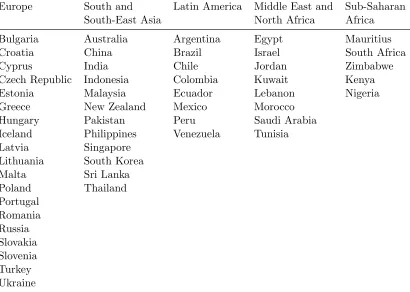
five regions: Europe, South and South-East Asia, Latin America, Middle East and North Africa, and Sub-Saharan Africa (see Table 2.3 for a list of countries by region). The neighbourhood matrix is defined as
wN bdij = PNδij h=1δih
whereδij takes the value 1 when countryiand countryjbelong to the same region, and
0 otherwise. Yuzefovich (2003) demonstrates that all the weight matrices are absolutely bounded in row and column sums. The diagonal elements are also normalised to zero. The common shocks are of two types: those propagated through trade linkages (in
FN) and those through financial linkages (in Xt,N). Suppose that
FN = (f1, . . . , fN)0, Xt,N = (xt,1, . . . , xt,N)0.
Then the common shocks used are
fi0 =
Exportsi,Europe
GDPi
,Exportsi,Japan
GDPi
,Exportsi,U S
GDPi
x0t,i =
bi,Europe
GDPi
yEurope,t,
bi,Japan
GDPi
yJapan,t, bi,U S
GDPi
yU S,t
whereExportsi,C and bi,C are the exports from country i to financial centre C while yC,t is the weekly stock market return in financial centre C at time t. Yuzefovich
(2003) suggests that thext,i may be endogenous but a Hausman test conducted by him
indicates otherwise and we treat them as exogenous, as he does in his final specification. The model estimated is therefore
yn = (IT ⊗lN)α+Xnβ+ (IT ⊗FN)γ+λ1
IT ⊗WT rade
yn
+ λ2 IT ⊗WF inyn+λ3 IT ⊗WSimyn
+ λ4
IT ⊗WN bd
yn+Un (2.5.1)
withk1=k2 = 3.
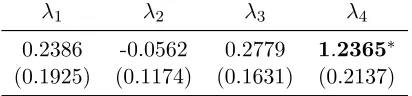
λ1 λ2 λ3 λ4
0.2386 -0.0562 0.2779 1.2365∗
[image:38.595.215.421.110.158.2](0.1925) (0.1174) (0.1631) (0.2137)
Table 2.1: Summary of estimates of coefficients corresponding to weighting matrices in specification (2.5.1)
Standard errors are reported in parentheses, starred estimates in bold are significant at 5% level
We now allow for different spatial parameters for different phases of the sampling period, as indicated in Section 2.4.2. In particular, we split the sampling period into three four-week periods, henceforth referred to as months. For the insignificant spatial lags, we find that the lags remain insignificant in each month even after allowing for different spatial parameters. As a result, we estimate the model with different spatial parameters for each month corresponding only to the significant financial links matrix. Specifically, the model estimated is:
yn = (IT ⊗lN)α+Xnβ+ (IT ⊗FN)γ+λ1
IT ⊗WT radeyn
+
3
X
j=1
λj2 IT ⊗WjF in
yn+λ3 IT ⊗WSim
yn
+ λ4
IT ⊗WN bd
yn+Un (2.5.2)
where
W1F in=diagWF in, WF in, WF in, WF in,0, . . . ,0
andW2F in and W3F in are defined analogously using the 5th-8th and 9th-12th diagonal
blocks respectively. IV estimation is used, with the linearly independent columns of
Xn, IT ⊗WT radeXn, IT ⊗WSimXn, IT ⊗WN bdXn, IT ⊗WjF inXn, j = 1,2,3
and
IT ⊗FN,
IT ⊗WT rade
(IT ⊗FN), IT ⊗WSim(IT ⊗FN),
IT ⊗WN bd
(IT ⊗FN), IT ⊗WjF in
(IT ⊗FN), j = 1,2,3
being used as instruments, so that rn from Section 2.3.1 may also be taken as T /4
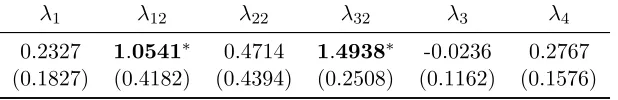
here. Table 2.2 reports the estimates of the spatial autoregressive parameters. These indicate thatλ12 and λ32 are significant at the 5% level, while λ22 is not. This would
λ1 λ12 λ22 λ32 λ3 λ4
0.2327 1.0541∗ 0.4714 1.4938∗ -0.0236 0.2767
[image:39.595.165.474.109.159.2](0.1827) (0.4182) (0.4394) (0.2508) (0.1162) (0.1576)
Table 2.2: Summary of estimates of coefficients corresponding to weighting matrices in specification (2.5.2)
Standard errors are reported in parentheses, starred estimates in bold are significant at 5% level
the fact that immediately after a crisis, country iimmediately increases its borrowing
from a financial centre but this stabilises after a few weeks. However some domestic businesses hit hard by the crisis may only start to feel financial hardship some time after the initial shock and create a second wave of demand for borrowing. At-test was
also conducted for the null hypothesis
H0 :λ12=λ32
which failed to reject the null returning a test statistic value of 0.9358, indicating that both ‘waves’ seem to have equal impact on stock market returns through the financial channel.
Remark In another piece of research, not published in this thesis, we consider the problem of testing increasingly many linear restrictions on the parameters θ(n) =
λ0(n), β(0n)0 of (2.2.1). Such a problem is natural not only because of the
increasing-parameter definition of the model, but also because the increasing autoregressive order can arise from a partitioning of the data (see Chapter 2). In the latter case, Chapter 2 prescribes an approach that takes into account heterogeneity between the clusters by recommending that the autoregressive parameters be allowed to vary across clusters. On the other hand, practitioners have a preference for a parsimonious model where possible. As a result there is great interest in testing null hypotheses of the type
H0 :λ1 =λ2=. . .=λpn. (2.5.3)
Bearing in mind that pnincreases with n, a more meaningful way of writing the above
null hypothesis would be
H0 :
pn
X
i,j=1
i<j
(λi−λj)2 = 0. (2.5.4)