2017 International Conference on Mathematics, Modelling and Simulation Technologies and Applications (MMSTA 2017) ISBN: 978-1-60595-530-8
GARCH-LSSVM Coupled Predication Model and Its Application
on Stock Index Forecasting
Xiao-xu HU
1,2, Meng-qi ZHANG
1,2and Xin JIANG
1,3,*1Key Laboratory of Mathematics, Informatics and Behavioral Science, Ministry of Education,
Beihang University, Beijing 100191, China;
2School of Mathematics and Systems Science, Beihang University, Beijing 100191, China;
3Beijing Advanced Innovation Center for Big Data and Brain Computing, Beijing 100191, China
*Corresponding author
Keywords: Generalized auto-regressive conditional heteroscedastic (GARCH), Least square support vector machine (LSSVM), Coupled prediction algorithm, Stock index forecasting, Technical indicators.
Abstract. It is usually a challenge for traditional time series prediction models to combine the linear and non-linear factors effectively, which might cause a problem that the trend forecast is not accurate. In this paper we propose a new prediction model based on GARCH and LSSVM. The GARCH model is used to deal with the heteroscedasticity of the residual series of the closing price of the stock index data. At the same time, a number of technical indicators are constructed to train the LSSVM model and the corresponding predicted values and residuals are obtained. Further, the predicted value and the residual obtained respectively from GARCH and LSSVM are used as the training set to modify the LSSVM model, with the predicted value of the logarithmic closing price of the stock index obtained. This coupled model not only contains the linear trend of historical information, but also integrates the non-linear features such as market volatility information which is closely related to the target data. Numerical experimental results show that the prediction accuracy of the model is 98.22% on the testing data set. This model performs also better than the GARCH 97.84% and the LSSVM 98.04% respectively in accuracy deviation.
Introduction
At present, how to build an efficient quantitative model to predict the price trend of securities has become a challenging and valuable work [1]. For the government macro management, accurately predicting the stock price index and stock price trend in the stock market can monitor and guide the smooth operation of the stock market at a certain level and reduce the market risk. For investors, building a quantitative model, has a good reference value for its effective investment strategy.CSI300 index is from Shanghai and Shenzhen two stock market 300 A shares as a sample compiled from the stock index and the stock market, as the representative of good, high liquidity, active trading ma-instream investment stocks, earnings can reflect the mainstream market investment. Therefore, the accurate prediction of CSI300 index has higher practical significance. For the prediction of time series, scholars have proposed many prediction models, including linear models and nonlinear models. Generalized auto-regressive conditional heteroscedastic (GAR- CH) is a linear regression model specially designed for financial data. Ferenstein and Gasowski (2004) used AR-GARCH to model stock data [2]. Chen and Hu (2011) studied traffic flow forecasting by means of ARIMA-GARCH model [3]. But GARCH model is just a linear model that cannot capture nonlinear components.
transform the quadratic program problem into linear equations. In this paper, we construct a GARCH-LSSVM coupled optimization model and establish the verification performance index, which combines the regularization parameter and the kernel parameter in the model to achieve the prediction of the CSI300 index price.
Basic theory GARCH Model
Most financial time series do not have the independent normal distribution characteristic, instead, they display peak thick tails, the negative bias and the characteristic clustering. In this case, the traditional econometric model is difficult to describe its fluctuation law, and the conditional heteroscedasticity model is needed. The ARCH model is considered as the most widely used conditional heteroscedasticity model that reflects the variance characteristics and is widely used in time series analysis of financial data. The mathematical idea of the ARCH model is as follows
t t t
Y
X
(1)
2 2 2
0 1 1... 1 2 3...
t a a t aq t q t t
, ,,(2)
where Yt is the explained variable,Xt is the explanatory variable,t is the residual sequence.
The ARCH model usually analyzes the stochastic perturbation terms of the subject model in order to extract the information from the residuals adequately, so that the final model residual t become white noise sequence. If the square of the error is represented by the ARMA model, the ARCH model is transformed into the GARCH model (Bollerslev, 1986), and the GARCH(p,q) model is
t t t
Y X
(3)
2 2 2
0
1 1
.
p q
t i t i j t j
i j
(4)
Here 2 2
1 1
1
p q
i t i j t j
i j
is restriction.LSSVM Model
LSSVM is an improved model of SVM, it changes the SVM inequality constraints into equality constraints. The error square and loss function are regarded as the empirical loss of the training set.so, the solution of the quadratic program is transformed into solving linear equations, improving calculation speed and convergence precision, reducing the difficulty of solving[5,6].
Given a training data set
1, n
i i i
x y , where xiRn is the input of the system, yiR is the
output of the system. The least squares support vector machine mathematical model is:
2, , 1
1
min ,
2 2
n T
i b
i
C J
The constraints in the formula are
= T ; 1, 2,...,
i i i
y
x b
i n (6)
is a nonlinear mapping which maps xi from the input space are mapped to highdimensional (even infinite dimensional) feature space, so as to realize the nonlinear regression in the input space into linear regression in high-dimensional feature space. By constructing the Lagrange function, the constraint optimization can be transformed into unconstrained optimization, and the optimization problem can be transformed into solving linear equations according to the KKT condition [7.8]:
1
0
0 T
v
v
b I
a y
I H c I
(7) wherey=[ , ,..., ]y y1 2 yn T, [1,1,...,1]
T v
I , [ , , ...,1 2 ]T
n
a a a a ,H={Hij i j, 1, 2,.., }n ,Hij=
T
,
i j i j
x x K x x
,K
is a kernel function.Coupling Model
This paper uses CSI300 index data from wind database (http://www.wind.com.cn) for empirical analysis, the time ranges from January 5, 2015 to June 30, 2017, with 607 samples. Each data sample includes five characteristics: the opening price, the highest price, the lowest price, volume, and amount. Select the above characteristics to construct seven indexes, which have strong correlations with closing price as the input vectors, the specific meaning is as follows. The output variable Y is the logarithmic closing price of the CSI300 index [9].
(1) VoluIndex: The ratio of today’s trading volume to the average daily trading volume of M
days
(2) CloseIndex: The ratio of today’s trading close to the average daily trading close of M days
(3) TrAmIndex: The ratio of today’s trading amount to the average daily trading amount of M
days
(4) MeanIndex: The average closing price for the past M days (5) RateChangeIndex: The ups and downs of past M days (6) HighIndex: The highest closing price of past M days (7) Lowdex:The lowest closing price of past M days
We apply window-type mobile standardization, which only uses the previous i-1 day mean and standard deviation to standardize the i-th day data:
' i i , 1, 2,... i
i
x x
x i
Var x
, (8)
where xi, Var x
i represents the mean and standard deviation of the sample starting point to thei-th day accordingly.
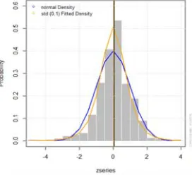
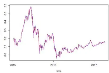
Figure 1. CSI300 index trend. Figure 2. CSI300 index distribution.
Before the application of the model, we carry out the corresponding statistical analysis on the feasibility of establishing the GARCH model forecasting for the index closing price series [11,12].
1. Smoothness test. After the unit root ADF test with R language, it shows that the logarithmic closing price of the CSI300 index is at a significant level of 1% of the test P-value of 0.249, greater than 0.01, indicating a non-stationary sequence. The P-value of the logarithmic yield sequence of the CSI300 index is much less than 0.01 and the probability that the logarithmic yield sequence has a unit root is almost zero. There should be no obvious memory and the persistence of volatility for the smooth sequence. We set up the GARCH model for the logarithmic yield sequence of the CSI300 index.
2. GARCH effect test. The ARCH-LM test of the logarithmic yield series of the CSI300 index indicates that the coefficients of the residual autoregressive function are distinct from zero, and the sequence still has significant autocorrelation, i.e., ARCH effect. In summary, the logarithmic yield series of CSI300 has obvious fluctuation aggregation, stable sequence, significant ARCH effect, and can be modeled by GARCH.
3. GARCH model results output. We use the ugarchspec function of rugarch package in R language to establish the GARCH model and optimize the CSI300 index logarithmic yield sequence, the ugarchfit function to fit the GARCH model. The predicted results show that the P-value of the output model coefficients is significantly zero. The model sGARCH (1, 1) can be well fitted to the historical logarithmic yield series of the CSI300 index. The model is as follows:
1 2 -1 -2
0.201
0.992
0.206
0.991
t t t t t t
y
y
y
(9)2 2 2
1 1
0.062 0.938
t t t
(10) 4. Model diagnosis. As can be seen from the histogram, the residual of the yield sequence satisfies the normal distribution. The Box-Ljung test shows that the autocorrelation values did not go beyond the significant (confidence) boundary in the lagged 1-20 order, and the P-value of the Box-Ljung test is 0.2619, indicating that the residuals are essentially white noise sequences. Therefore, the GARCH model is valid. [image:4.612.310.470.583.703.2][image:4.612.141.277.585.709.2]
The kernel function of the LSSVM model is a radial basis function:
,
=exp || ||2
2 2
i j i j
K x x x x (11)
a and b in the linear equation (7) can be obtained by least squares, the linear regression function is:
1
= n iK , i
i
f x a x x b
(12) where n is the number of input samples, x is the input variable,ai is not equal to zero. The inputsamplexi is the support vector, and a is support vector coefficient [13].
10% cross validation method is selected when parameter optimization is done in LSSVM model. The data set is randomly divided into 10 disjoint sub-datasets, of which seven sub-datasets contains 61 observations, 3 datasets contains 60 observations. In the subsequent 10 trials, each sub-datasets is taken as a test sample for each test and samples from the remaining nine sub-sub-datasets are used as training samples. First, given the kernel parameters, we minimize the RMES to select the regularization parameter C in a certain range with a RBI method. According to the selected regularization parameters, using the RBI method to minimize the RMES to select the kernel parameter sigma, we select the last parameter, which is the optimal combination of parameters, to test the test sample [14, 15].
The GARCH-LSSVM coupling prediction algorithm is as follows. Input: training sample set
,
l 1i i i
x y , where yiRis the log closing price, xi=
xi,1,xi,2,...,xi N,
is the eigenvalue of the discrete feature set A=
a a1, 2,...,aN
associated with the target yi and theinputxt+1=
xt1,1,xt1,2, ...,xt1,N
N 7
.Output: forecasting resultyt1.
Step 1. The historical opening price, the highest price, the lowest price, the volume and the amount of the sample CSI300 index are combined to obtain seven indicators with high correlation with the index closing price, which is denoted as discrete numerical feature set A.
Step2. Normalize the feature set A by window movement, i.e.,
' i i , 1, 2,... i
i
x x
x i
Var x
the
CSI300’s closing price sequence is logarized to get the sequenceyi.
Step3.The GARCH model is established for the logarithmic yield series of the sample CSI300 index, and then the GARCH model is used to obtain the fitted value of the logarithmic closing price series, noting asY1, according to formula e' yiY1,we get the residual sequence, noting as r1.
Step4.Train the LSSVM on the training set, use the radial basis function, and select the optimal parameters of the LSSVM with the 10-fold cross validation method. Where the eigenvector
Is 7 dimension input variables standardized. That is, the result of the standardization is highly correlated with the closing price.
Step5.In the trained LSSVM model to get the fitting results of training set, noting as
2
Y .according to formulae, we get the residual sequence, noting as r2.
Step6.the fitting numbersY1, Y2 and the residual value sequencesr1, r2 can be obtained from step3 and step5 as the input variables of the LSSVM model, logarithmic closing as an output variable, training model.
Step7.Add xt+1=
xt1,1,xt1,2,...,xt1,N
into step3 and step5 respectively, we get the fittingvalues 1
1
t
y ,yt21,the residual values 1
1
t
r ,rt21.
Figure 5. Coupling model fitting effect diagram.
The indicators used here to evaluate the performance of different predictive models are Root Mean Square Errors (RMSE),Relative Square Error(RSE) and Rsquare. Different model performan- ce indicators as shown below, we can see that the performance of the coupling model is superior to a single GARCH model and LSSVM model.
Table 1. Comparison of model performance.
Model
Insample Outsample
RMSE RSE Rsquare RMSE RSE Rsquare GARCH 0.0191 0.0216 0.9784 0.0267 0.0938 0.9062 LSSVM 0.0182 0.0196 0.9804 0.0218 0.0803 0.9197 GARCH- LSSVM 0.0174 0.0178 0.9822 0.0209 0.0607 0.9393
Conclusion
Generally, GARCH model cannot effectively analyze the core nonlinear features of time series, in order to solve the problem, we study the nonlinear deviation of GARCH based on the LSSVM model with strong nonlinear predictive ability and generalization ability, and then train the model of the prediction of non-linear volatility pattern recognition. Meanwhile, the GARCH-LSSVM coupled forecasting model is proposed, and the over-fitting of non-linear terms by heteroscedasticity of the GARCH model is corrected. How to consider more core factors in the process of model training and further optimize the related parameters of LSSVM is the focus and direction of the next step.
Acknowledgments
This work is supported by NSFC (Grants No. 11201017, 11290141) and National Key Research and Development Program of China (Grant No. 2017YFB0701702).
References
[1] Peng T., Tang Z., A small scale forecasting algorithm for network traffic based on relevant local least squares support vector machine regression model, J. Appl. Math 2015, 9, 653–659. [2] E. Ferenstein, M. Gasowski, Modelling stock returns with AR-GARCH processes, J. SORT-Statistics and Operations Research Transactions, 2004, 28(1): 55-68.
[3] Chen C., Hu J., Meng Q., et al. Short-time traffic flow prediction with ARIMA-GARCH model, C. Intelligent Vehicles Symposium (IV), IEEE, 2011: 607-612.
[4] J.A.K. Suykens, J. Vandewalle, Least squares support vector machine classifiers, J. Neural Processing Letters, 1999, 9(3): 293-300.
[image:6.612.128.488.289.357.2][6] Chung S.S., Zhang S. Volatility estimation using support vector machine: Applications to major foreign exchange rates, J. Electronic Journal of Applied Statistical Analysis, 2017, 10(2): 499-511.
[7] Zhang Y., Dong Z., Liu A., et al. Magnetic resonance brain image classification via stationary wavelet transform and generalized eigenvalue proximal support vector machine, J. Journal of Medical Imaging and Health Informatics, 2015, 5(7): 1395-1403.
[8] Wu Q., Peng C. Wind power generation forecasting using least squares support vector machine combined with ensemble empirical mode decomposition, principal component analysis and a bat algorithm, J. Energies, 2016, 9(4): 261.
[9] Zhu B., Han D., Wang P., et al. Forecasting carbon price using empirical mode decomposition and evolutionary least squares support vector regression, J. Applied Energy, 2017, 191: 521-530. [10] Lai L., Liu J. Support Vector Machine and Least Square Support Vector Machine Stock Forecasting Models, J. Computer Science and Information Technology, 2014, 2(1): 30-39.
[11] J. Contreras, Y.E. Rodríguez. GARCH-based put option valuation to maximize benefit of wind investors, J. Applied Energy, 2014, 136(C): 259-268.
[12] Badescu, R. J. Elliott, J.P. Ortega, Non-Gaussian GARCH option pricing models and their diffusion limits, J. European Journal of Operational Research, 2015, 247(3): 820-830.
[13] Ou P., Wang H. Financial Volatility Forecasting by Least Square Support Vector Machine Based on GARCH, EGARCH and GJR Models: Evidence from ASEAN Stock Markets, J. International Journal of Economics & Finance, 2010, 2(1): 337-367.