Munich Personal RePEc Archive
A test for model specification of diffusion
processes
Chen, Song Xi and Gao, Jiti and Tang, Chenghong
Iowa State University, The University of Adelaide, Iowa State
University
November 2005
Online at
https://mpra.ub.uni-muenchen.de/11976/
A Test for Model Specification of Diffusion Processes
Song Xi Chen and Jiti Gao
Iowa State University and The University of Western Australia
Abstract: This paper evaluates the use of the nonparametric kernel method for
testing specification of diffusion models as originally considered in A¨ıt-Sahalia (1996).
A serious doubt on the ability of the kernel method for diffusion model testing has
been cast in Pritsker (1998), who observes severe size distortion of the test proposed
by A¨ıt-Sahalia and finds that 2755 years of data are required in order for the kernel
density estimator to attain a level of accuracy achieved with 22 years of independent
data. We introduce in this paper a set of measures to formulate a new test based on the
kernel method and show that the severe size distortion observed by Pritsker (1998) can
be overcome. The meaures include targeting at the transitional desnity of the process,
using the empirical likelihood to formulate the test statistics, properly smoothing of
model-implied transtional densities and employing a parametric bootstrap procedure
in approximating the distribution of test statistics. Our simulation for both the
Vasicek and Cox-Ingersoll-Ross diffusion models indicates that the proposed test has
reasonable size and power under various degrees of data dependence for as little as 10
years of data. We then apply the proposed test to a monthly Federal Fund rate data
and find that there is some empirical support for several of the one-factor diffusion
models proposed in the literature.
KEYWORDS: Bootstrap, Continuous–time interest rate model, Diffusion process,
1. Introduction. Let X1,· · ·Xn+1 be n+ 1 equally spaced (with spacing ∆ in
time) observations of a diffusion process
dXt =µ(Xt)dt+σ(Xt)dBt (1.1)
whereµ(·) andσ2(·)>0 are, respectively, the drift and diffusion functions, and B t is
the standard Brownian motion. Suppose a parametric specification of model (1.1) is
dXt =µ(Xt;θ)dt+σ(Xt;θ)dBt, (1.2)
whereθ is a parameter within a parameter space Θ⊂Rd for a positive integerd. The
focus of this paper is testing the validity of the parametric specification (1.2) based
on the discretely observed data{Xt}n+1t=1.
In a pioneer work that represents a major break-through in financial
economet-rics, A¨ıt-Sahalia (1996) proposes using the nonparametric kernel method to test the
parametric specification (1.2). The test statistic is aL2–distance between the kernel
stationary density estimator and the stationary density implied by model (1.2). The
test is based on the asymptotic normal distribution of the test statistic.
In a comprehensive investigation, Pritsker (1998) evaluates A¨ıt-Sahalia’s test and
finds a large discrepancy between the simulated and nominal sizes of the test under
a set of Vasicek (1977) diffusion models with various degrees of dependence. He
observes that both the form of the density estimator and its asymptotic distribution
are the same for both independent and dependent observations, which is due to the
so-called ‘pre-whitening’ by a smoothing bandwidth in nonparametric curve estimation.
Hence, the asymptotic nature of the A¨ıt-Sahalia’s test prevents capturing dependence
existed in the process. Pritsker shows that to attain the same level of accuracy for
the kernel estimator with 22 years of independent data would require 2755 years of
dependent data under the Vasicek model. In a separate study, Chapman and Pearson
the boundary and truncation bias associated with the kernel regression estimator.
These findings have illustrated the challenge when applying the kernel estimator for
inference of diffusion processes, and have inevitably projected rather negatively on
the ability of the kernel method to model data dependence induced by a diffusion
process in general and testing of the diffusion process in particular.
We think other aspects contribute to the performance of A¨ıt-Sahalia’ test in
addi-tion to its asymptotic nature observed by Pritsker. One is that the test targeted at the
stationary density. It can take long time for a process to settle on the stationary
dis-tribution which is specially the case for the Vasicek models with weak mean-reversion
considered in Pritsker’s simulation. As pointed out in A¨ıt-Sahalia (1996), a test on
the stationary density is not conclusive as two different processes may share the same
stationary density. As diffusion processes are Markovian, testing should be aimed at
the transitional density. The second aspect is that the kernel estimator introduces a
bias which needs to be considered. A¨ıt-Sahalia proposed undersmoothing to prevent
the bias from getting into the limiting distribution. However, it may not be easy to
check on the effect of a particular bandwidth used on the bias. Another aspect is
that parameter estimates under the hypothesized process are needed in the
formu-lation of a test statistic. However, the maximum likelihood estimators for the drift
parameters are subject to large bias when the process is weak mean-reverting. This
is a well–known problem in diffusion process estimation (Yu and Phillips, 2001) and
further reduces the performance of A¨ıt-Sahalia’s test.
We implement a set of measures in developing a new test based on the kernel
method. First of all, the proposed test is targeted at the transitional density to
have a conclusive test and to fully capture the dynamics. The second measure is
to properly smooth the model implied transitional density so as to cancel out the
the theoretical analysis. In order to put the difference between the kernel estimator
and the smoothed model-implied transitional density in the context of its variation,
the test statistic is formulated via the empirical likelihood of Owen (1988, 1990).
Furthermore, to make the test robust against bandwidth choice, we formulate the
test statistic based a set of bandwidths. Finally, a parametric bootstrap procedure is
used to profile the distribution of the test statistic and to obtain the critical value of
the test.
A continuous-time diffusion process and a time series model share some important
features althought one is a continuous time model and the other is a discrete model.
Time series and diffusion processes can be both Markovian and weakly dependent
satisfying certain mixing conditions. Kernel–based tests have been shown to be able
to effectively test for discrete time series models as demonstrated in Robinson (1989),
Hjellvik and Tjøstheim (1995), Fan and Li (1996), Hjellvik and Yao and Tjøstheim
(1998), Kreiss, Neumann and Yao (1998), Li (1999), A¨ıt-Sahalia, Bickel and Stoker
(2001), Gozalo and Linton (2001). See the books by Hart (1997) and Fan and Yao
(2003) for extended lists of references. For estimation of diffusion models, in
addi-tion to A¨ıt-Sahalia (1996) and Stanton (1997), Jiang and Knight (1997) proposed a
semiparametric kernel estimator for the drift. Fan, Jiang, Zhang and Zhou (2003)
examined effects of high order stochastic expansions. Bandi and Phillips (2003)
con-sider a two–stage kernel estimation procedure for the drift and diffusion functions
without the strictly stationary assumption. For testing of diffusion processes, Hong
and Li (2005) developed a test via a conditional probability integral transformation.
Although the kernel estimator is employed, the transformation leads to
asymptot-ically independent uniform random variables under the correct model. Hence, the
issue on the ability of the kernel method to model dependence induced by diffusion
for the drift and diffusion functions. See review articles by Cai and Hong (2003) and
Fan (2005) for more detailed accounts.
The paper is structured as follows. Section 2 outlines the hypotheses and the kernel
estimation of the transitional densities. The proposed EL test is given in Section 3.
Section 4 reports main results of the test. Section 5 considers computational issues.
Results from simulation studies are reported in Section 6. A Federal fund rate data
is analyzed in Section 7. All the proofs are given in the appendix.
2. The hypotheses and kernel estimators. Letπ(x) be the stationary density
andp(y|x; ∆) be the transitional density ofXt+1 =ygivenXt=xunder model (1.1)
respectively; andπθ(x) andpθ(y|x,∆) be their parametric counterparts under model
(1.2). To simplify notation, we suppress ∆ in the notation of the transitional densities.
LetX be the state space of the process.
Although πθ(x) has a close form expression via Kolmogorov forward equation
πθ(x) =
ξ(θ)
σ2(x, θ)exp
x
x0
2µ(t, θ)
σ2(t, θ)dt
,
where ξ(θ) is a normalizing constant, pθ(y|x) implicitly defined by the Kolmogorov
backward-equation may not admit a close form expression. However, this problem is
overcome by Edgeworth type approximations developed by A¨ıt-Sahalia (1999, 2002)
for general diffusion processes. As the transitional density fully describes the
dynam-ics of a diffusion process, the hypotheses we would like to test are
H0 :p(y|x) =pθ0(y|x) for some θ0 ∈Θ and all (x, y)∈S ⊂ X
2 versus
H1 :p(y|x)=pθ(y|x) for allθ ∈Θ and some (x, y)∈S ⊂ X2, (2.1)
where S is a compact set within X2 and can be chosen upon given observations
as demonstrated in simulation and case studies in Sections 6 and 7. As we choose
estimators (M¨uller, 1991; Fan and Gijbles, 1996; and M¨uller and Stadtm¨uller, 1999)
is avoided.
Let K(·) be a kernel function which is a symmetric probability density function,
h is a smoothing bandwidth such that h → 0 and nh2 → ∞ as n → ∞, and
Kh(·) =h−1K(·/h). The kernel estimator of p(y|x) is
ˆ
p(y|x) =n−1 n
t=1
Kh(x−Xt)Kh(y−Xt+1)/πˆ(x). (2.2)
where ˆπ(x) = (n+ 1)−1n+1
t=1 Kh(x−Xt) is the kernel estimator of the stationary
density used in A¨ıt-Sahalia(1996). The local polynomial estimator introduced by Fan,
Yao and Tong (1996) can be also employed without altering the main results of the
paper. It is known (Hydman and Yao, 2002) that
E{pˆ(y|x)−p(y|x)} = 1 2σ
2 kh2
∂2p(y|x)
∂x2 +
∂2p(y|x) ∂y2 + 2
π′(x)
π(x) ∂p(y|x)
∂x
+o(h2) and(2.3)
Var{pˆ(y|x)} = R
2(K)p(y|x)
nh2π(x) (1 +o(1)), (2.4)
where σ2
K = u2K(u)du and R(K) = K2(u)du.
Let ˜θ be a √n–consistent estimator of θ under model (1.2) for instance the
maxi-mum likelihood estimator underH0, and
wt(x) =Kh(x−Xt)
s2h(x)−s1h(x)(x−Xt) s2h(x)s0h(x)−s21h(x)
(2.5)
be the local linear weight withsrh(x) = ns=1Kh(x−Xs)(x−Xs)l for r = 0,1 and
2. In order to cancel the bias in ˆp(y|x), we smooth pθ˜(y|x) as
˜
pθ˜(y|x) =
n+1
t=1 Kh(x−Xt) n+1
s=1 ws(y)pθ˜(Xs|Xt) n+1
t=1 Kh(x−Xt)
. (2.6)
Here we apply the kernel smoothing twice: first for each Xt using the local linear
weight to smoothpθ˜(Xs|Xt) and then employing the standard kernel weight to smooth
(1993). It can be shown following the standard derivations as those demonstrated in
Fan and Gijbels (1996) that, underH0
E{pˆ(y|x)−p˜θ˜(y|x)} = o(h2) and (2.7)
Var{pˆ(y|x)−p˜θ˜(y|x)} = Var{pˆ(y|x)}{1 +o(1)}. (2.8)
Hence the bias of ˆp(y|x) cancels that of ˜pθ˜(y|x) in the leading order whileas smoothing
the parametric density does not effect the asymptotic variance.
3. Formulation of a test statistic. The test statistic is formulated by the
empirical likelihood (EL) (Owen, 1988, 1990). Despite its being intrinsically
non-parametric, EL posesses two key properties of a parametric likelihood: the Wilks’
theorem and Bartlett correction. Qin and Lawless (1994) established EL for
parame-ters defined by generalized estimating equations which is the broadest framework for
EL formulation, which was extended by Kitamura (1997) to dependent observations.
Chen and Cui (2004) show that the EL admits Bartlett correction under this general
framework. An extension of Qin and Lawless’s framework is given in Hjort, McKeague
and Van Keilegom (2005) to include nuisance parameters/functions. Fan and Zhang
(2004) propose a sieve EL test for varying-coefficient regression model that extends
the test of Fan, Zhang and Zhang (2001). Tripathi and Kitamura (2003) propose an
EL test for conditional moment restrictions. See also Li and Van Keilegom (2002)
and Li (2003) for EL goodness-of-fit tests for survival data.
Let us now formulate the EL for the transitional density at a fixed (x, y). For
t = 1,· · ·, n, let qt(x, y) be non-negative weights allocated to (Xt, Xt+1). The EL
evaluated at ˜pθ˜(y|x) is
L{pˆθ˜(y|x)}= max n
t=1
qt(x, y) (3.1)
subject ton
t=1qt(x, y) = 1 and n
t=1
By introducing a Lagrange multiplierλ(x, y), the optimal weights as solutions to
(3.1) and (3.2) are
qt(x, y) =n−1{1 +λ(x, y)Tt(x, y)}−1, (3.3)
where Tt(x, y) =Kh(x−Xt)Kh(y−Xt+1)−p˜θ˜(x, y) andλ(x, y) is the root of
n
t=1
Tt(x, y)
1 +λ(x, y)Tt(x, y)
= 0. (3.4)
The overall maximum EL is achieved atqt(x, y) =n−1 which maximize (3.1) without
the constraint (3.2). Hence, the log-EL ratio is
ℓ{p˜θ˜(y|x)}=−2 log ([L{p˜θ˜(y|x)}nn]) = 2
log{1 +λ(x, y)Tt(x, y)}. (3.5)
It may be shown by similar derivations to those given in Chen, H¨ardle and Li (2003)
that
sup
(x,y)∈S|
λ(x, y)|=op{(nh2)−1/2log(n)}. (3.6)
Let ¯U1(x, y) = (nh2)−1Tt(x, y) and ¯U2(x, y) = (nh2)−1Tt2(x, y). From (3.4) and
(3.6), λ(x, y) = ¯U1(x, y) ¯U2−1(x, y) +Op{(nh2)−1log2(n)} uniformly with respect to
(x, y)∈S. This then leads to
ℓ{p˜θ˜(y|x)} = nh2U¯12(x, y) ¯U2−1(x, y) +Op{n−1/2h−1/2log3(n)}
= nh2{pˆ(y|x)−p˜θ˜(y|x)} 2
V(y|x) +Op{h
2+n−1/2h−1/2log3(n)
} (3.7)
uniformly for (x, y) ∈ S, where V(y|x) = R2(K)p(y|x)π−1(x). Hence, the EL
ratio is a studentized local goodness-of-fit measure between ˆp(y|x) and ˜pθ˜(y|x) as
Var{pˆ(y|x)}= Vnh(y|2x).
Integrating the EL ratio with a weight function ω(·,·) supported on S, the global
goodness–of–fit measure based on a single bandwidth is
N(h) =
To make the test less dependent on a single h, we extendN(h) over a bandwidth
setH ={hk}Jk=1wherehk+1/hk =afor somea∈(0,1), whose choice can be guided by
the cross-validation method of Fan and Yim (2005). This formulation is motivated by
Horowitz and Spokoiny (2001) who considered achieving the optimal convergence rate
of the local alternative hypothesis in testing regression models. A similar approach
was applied in Fan (1996) using wavelets.
The final test statistic that bases on the bandwidth set H is
Ln = max 1≤k≤J
N(h)−1
√
2h .
The standardization reflects that Var [N(h)] =O(2h2) as elaborated in the appendix.
4. Main Results. This section establish both asymptotic distribution and
asymptotic consistency forLn. In order to state the main results, we need to introduce
the following conditions.
Assumption 1. (i) Assume that the process {Xt} is strictly stationary and α
-mixing with the -mixing coefficient α(t) = Cααt defined by α(t) = sup{|P(A∩B)−
P(A)P(B)| :A ∈Ωs
1, B ∈ Ω∞s+t} for all s, t≥ 1, where 0 < Cα <∞ and 0 < α < 1
are constants, and Ωji denotes the σ-field generated by {Xt:i≤t≤j}.
(ii) K(·) is a bounded symmetric probability density supported on [−1,1]and has
bounded second derivative; and let σ2
K =: −∞∞ x2K(x)dx and R(K) =: −∞∞ K2(x)dx.
(iii) The bandwidth set H =
hk =hmaxak, k= 0,1,2, . . . , J
, where 0< a < 1,
h1 = cminn−γ1 and hmax =hJ = cmaxn−γ2, in which 17 < γ2 ≤ γ1 < 12, cmin and cmax
are constants satisfying 0< cmin, cmax<∞, and J is an integer not depending on n.
(iv) ω(x, y)is a bounded probability density supported on S.
Assumption 2. (i) Each of the diffusion processes given in (1.1) and (1.2)
time. In addition, each of the processes possesses a transitional density with p(y|x) =
p(y|x,∆)for model (1.1) and pθ(y|x) = pθ(y|x,∆)for model (1.2), respectively.
(ii) Let ps1,s2,···,sl(·) be the joint probability density of (X1+s1, . . . , X1+sl) (1≤ l ≤
6). Assume that each ps1,τ2,···,sl(x)is three times differentiable inx∈ X
l for1≤l≤6.
(iii) The parameter space Θ is an open subset of Rd and p
θ(y|x) is three times
differentiable in θ ∈ Θ. For every θ ∈ Θ, µ(x;θ) and σ2(x;θ), and µ(x) and σ2(x)
are all three times continuously differentiable inx∈ X, and both σ(x)andσ(x;θ)are
positive for x∈S and θ ∈Θ.
Assumption 3. (i)There is a positive and integrable function G(x, y) satisfying
E[max1≤t≤nG(Xt, Xt+1)] < ∞ uniformly in n ≥ 1 such that supθ∈Θ|pθ(y|x)|2 ≤
G(x, y)and supθ∈Θ|| ▽ j
θpθ(y|x)||2 ≤G(x, y) forj = 1,2,3, where ▽θpθ(·|·) = ∂pθ∂θ(·|·), ▽2
θpθ(·|·) = ∂ 2pθ(·|·)
(∂θ)2 and ▽3θpθ(·|·) = ∂ 3pθ(·|·) (∂θ)3 .
(ii)p(y|x)> c1 >0for all(x, y)∈S and that the stationary densityπ(x)> c2 >0
for all x∈Sx which is the projection of S on X for some ci >0 i= 1,2.
(iii)there is a finite C > 0 such that for every ε >0
E
inf
θ,θ′∈Θ:||θ−θ′||≥ε [pθ(Xt+1|Xt)−pθ
′(Xt+1|Xt)]
2
≥Cε2.
Assumption 4. (i)LetH0 be true. There exists aθ0 ∈Θsuch thatE
||θ˜−θ0||2
≤
C1Ln−1 for all sufficiently large n and a suitable constant C1L>0.
(ii)Let H1 be true. Then there is a θ1 ∈Θ such that E
||θ˜−θ∗||2≤C
2Ln−1 for
all sufficiently large n and a suitable constant C1L>0.
Assumption 1(i) imposes the strict stationarity and the α–mixing condition on
{Xt}. Under certain conditions, such as Assumption A2 of A¨ıt-Sahalia (1996) and
Conditions (A4) and (A5) of Genon–Catalot, Jeantheau and Lar´edo (2000),
Assump-tion 1(i) holds. AssumpAssump-tion 1(ii)(iii) is a quite standard condiAssump-tion imposed in kernel
estimation. Assumption 2 is needed to ensure the existence and uniqueness of a
may be implied under Assumptions 1–3 of A¨ıt-Sahalia (2002), which also cover
non-stationary cases. For the non-stationary case, Assumptions A0 and A1 of A¨ıt-Sahalia
(1996) ensure the existence and uniqueness of a stationary solution of the diffusion
process. Assumption 3 imposes additional conditions to ensure the smoothness of
the transitional density and the identifiability of the parametric transitional density.
Assumption 4(i) requires the usual rate of convergence for ˜θ to θ0. Such a rate is
achievable when ˜θ is the maximum likelihood estimator. The θ∗ in Assumption 4(ii)
can be regarded as a projection of the parameter estimator ˜θ under H1 onto the null
parameter space.
Let K(2)(z, c) = K(u)K(z+cu)du be a generalization to the convolution of K,
ν(t) = {K(2)(tu, t)}2
du {K(2)(v, t)}2
dvand ΣJ = R42(K)
ω2(x, y)dxdy(ν(ai−j)) J×J
be a J×J matrix where a is the fixed factor used in the construction ofH.
Further-more, Let 1J be aJ-dimensional vector of ones andβ = C(K)R(K)1
p(x,y)
π(y) ω(x, y)dxdy.
We now state the following asymptotic normality; its proof is given in Appendix
A.
Theorem 1. Under Assumptions 1–4 and H0, Ln d
→ max1≤k≤JZk as n → ∞
where Z = (Z1, . . . , ZJ)T ∼N(β1J,ΣJ).
Theorem 1 brings a little surprise in that the mean of Z is non-zero. This is
because, although the variance of ˜pθ(x, y) is at a smaller order than that of ˆp(x, y), it
contributes to the second order mean ofN(h) which emerges after the standardization.
However, this will not affect the test as shown in Theorem 2.
We are reluctant to formulate a test based on Theorem 1 as such a test would be
slow converging too. Instead we propose the following parametric bootstrap procedure
to approximatelα, the 1−αquantile ofLnwhereα∈(0,1) is the nominal significance
Step 1: Generate an initial value X∗
0 from the estimated stationary densityπθ˜(·).
Then simulate a sample path {X∗
t}n+1t=1 at the same frequency ∆ according to dXt = µ(Xt; ˜θ)dt+σ(Xt; ˜θ)dBt.
Step 2: Let ˜θ∗ be the estimate ofθ based on{X∗
t}n+1t=1. Compute the test statistic Ln based on the resampled path and denote it byL∗n.
Step 3: For a large positive integer B, repeat Steps 1 and 2 B times and obtain
after rankingL1∗
n ≤L2n∗ ≤ · · · ≤LBn∗.
Let l∗
α be the 1−α quantile of L∗n satisfyingP
L∗
n ≥lα∗|{Xt}n+1t=1
=α. A Monte
Carlo approximation ofl∗
α isL
[B(1−α)]+1∗
n . The proposed test rejects H0 if Ln≥lα∗.
The next theorem shows that the proposed EL test based on the bootstrap
calibra-tion has correct size asymptotically and is consistent. The proof is given in Appendix
A.
Theorem 2. Under Assumptions 1–4, then limn→∞P(Ln ≥lα∗) = α under H0;
and limn→∞P (Ln ≥l∗α) = 1 under H1.
5. Computation. The computation of the test statistic Ln involves first
com-puting the EL ratio ℓ{p˜θˆ(y|x)} over a grid of (x, y)-points within the set S ⊂ X2.
Then, N(h) in (3.8) is computed by its Riemann sum over a set of grid points in S
upon given the weight functionω(·,·). The EL test statistic Ln is obtained by taking
the maximum of N(h) over h ∈ Hn. The critical value lα is approximated via the
bootstrap procedure.
Despite being computationally intensive in each of these steps, implementing the
proposed test for a single data set is not a problem with a standard computing capacity
these days. However, when carrying out simulations, we would like to speed up the
computation as a large number of replications are required.
In the simulation, we use the least squares empirical likelihood (LSEL) to replace
closed-form solutions for the weights qt(x, y) and hence avoids expensive nonlinear
optimization. The log LSEL ratio evaluated at ˜pθ˜(y|x) is
lsl{p˜θ˜(y|x)}= min n
t=1
{nqt(x, y)−1}2
subject to n
t=1qt(x, y) = 1 and
n
t=1qt(x, y)Tt(x, y) = 0. According to Brown and
Chen (1998), the LSEL weights are given by
qt(x, y) =n−1+{n−1T(x, y)−Tt(x, y)}τS−1(x)T(x, y)
where T(x, y) =n
t=1Tt(x, y) and S(x, y) = n−1
n
t=1Tt2(x, y). And
lsl{m˜θ˜(x)}=S−1(x, y)T2(x, y)
is readily computable. The LSEL counterpart toN(h) isNls(h) = lsl{m˜ ˜
θ(x)}π(x, y)dx.
The final test statistic Ln = maxh∈H N
ls(h)−1
C(K)h . It can be shown from Brown and
Chen (1998) thatNls(h) and N(h) are equivalent to the first order. Therefore, those
first-order results in Theorems 1 and 2 continue to hold for the LSEL.
6. Simulation studies. We report results of simulation studies which designed
to evaluate the empirical performance of the proposed EL test. To gain information
on its relative performance, Hong and Li’s test is performed over the same simulation.
Throughout the paper, the biweight kernel K(u) = 1516(1−u2)2I(|u| ≤ 1) was
used in all the kernel estimation. In simulation, we set ∆ = 121 implying monthly
observations which coincides with that of the Federal fund rate data to be analyzed.
We chose n = 125,250 or 500 respectively corresponding roughly 10 to 40 years of
data. The number of simulations was 500 and the number of bootstrap resampled
paths was B = 250.
6.1. Size Evaluation.
Two simulation studies were carried out to evaluate the size of the proposed test.
second study three Cox, Ingersoll and Ross (CIR) (1985) models are considered. We
want to see if the severe size distortion observed by Pritsker (1998) is present for our
proposal.
6.1.1 Vasicek Models
We first consider, like Pritsker (1998), testing the Vasicek model
dXt =κ(α−Xt)dt+σdBt.
The vector of parameters θ = (α, κ, σ2) takes three sets of values which correspond
to Model -2, Model 0 and Model 2 of Pritsker (1998). The baseline Model 0 assigns
κ0 = 0.85837, α0 = 0.089102 and σ02 = 0.0021854 which matches estimates by
A¨ıt-Sahalia (1996) for an interest rate data. Model -2 is obtained by quadruplingk0 and
σ2
0 and Model 2 by halvingk0 andσ02 twice while keepingα0 unchanged. These three
models were part of the five models used in Pritsker (1998). Note that the three
models have the same marginal distribution N(α0, VE), where VE = σ 2
2κ = 0.01226
is the same. Despite the stationary distribution being the same, the models offer
different levels of dependence as quantified by the mean-reverting parameterκ. From
Models -2 to 2, the process becomes more dependent as κ gets smaller. This is
carefully designed by Pritsker to allow the effects of dependence to be investigated
without changing the marginal density.
The regionS was chosen based on the underlying transitional density so that the
region attained more than 90% of the probability. In particular, for Models -2, 0 and
2, it was chosen by rotating respectively [0.035,0.25] × [−0.03,0.03], [0.03,0.22] ×
[−0.02,0.02] and [0.02,0.22]×[−0.009,0.009] 45 degrees anticlock-wise. The weight
function ω(x, y) = |S|−1I{(x, y)∈S} where|S| is the area of S.
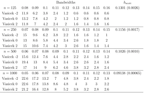
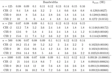
Both the cross-validation (CV) (Silverman 1986) and the reference to a bivariate
selection of the bandwidth setH whose values are reported in Table 1. Table 1 also
contains the average bandwidths obtained by the two methods. We observed that,
for each givenn, regardless of which method was used, the chosen bandwidth became
smaller as the model was shifted from Model -2 to Model 2. This indicated that
both methods took into account the changing level of dependence induced by these
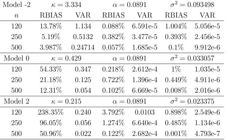
models. The maximum likelihood estimator was used to estimateθ in each simulation
and each resample in the bootstrap. Table 2 summarizes the quality of the parameter
estimation.
The average sizes of the proposed test at the nominal size of 5% are reported
in Table 3. It shows that the sizes of the proposed test were quite close to the
nominal level for Vasicek Model -2 and Model 0 consistently for the three sample
sizes considered. For Model 2, which has the weakest mean-reversion, there was
some size distortion when n = 125. However, it was significantly alleviated when n
was increased. The message conveyed by Table 3 is that we need not have a large
number of years of data in order to achieve a reasonable size for the test. Table 3 also
reports the single-bandwidth based test based onN(h) and the asymptotic normality
as conveyed by Theorem 1 with J = 1. Like Pritsker’s study, this asymptotic test
has severe size distortion too and highlights the need for implementing the bootstrap
procedure.
The size distortion for Model 2 at n = 125 was partly due to the poor quality of
parameter estimates. It is well known that the estimation of κ is subject to severe
bias when the mean-reversion is weak. This is indeed confirmed in Table 2. The
deterioration in the quality of the estimates, especially for κ when the dependence
became stronger, is alarming. The relative bias of the κ-estimates was more than
200% for Model 2 atn= 125. It is nice to see that the proposed test did a very good
the proposed test is robust against poor parameter estimates.
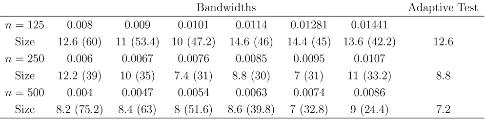
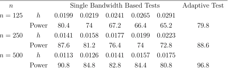
We also carried out simulation for the test of Hong and Li (2005). The Scott rule
adopted by Hong and Li was used to get an initial bandwidth (hscott). We then chose
4 equally spaced bandwidths below and above the average hscott. The nominal 5%
test at each bandwidth was carried out with the lag values 1 and 4. We only report
the results for lage value 1 in Table 4 as those for the other case were the same.
For sample size not larger than 500, the sizes of the test did not settle well at the
nominal level as reflected by the sizes being quite high for smaller bandwidths and
then dropped quite quickly for larger bandwidths. The performance may be due to a
combination of (i) the varying quality in parameter estimation as reported in Table
2 may affect the nature of the transformed series and (ii) the slow convergence to
normality of the test statistic.
6.1.2 CIR Models
We then conduct simulation on three CIR models to see if the pattern of results
observed for the Vasicek models holds for the CIR models. The CIR models are
dXt =κ(α−Xt)dt+σ
XtdBt, (6.1)
where the parameters were: κ= 0.89218, α= 0.09045 andσ2 = 0.032742 in the first
model (CIR 0); κ = 0.44609, α = 0.09045 and σ2 = 0.16371 in model CIR 1 and
κ = 0.22305, α = 0.09045 and σ2 = 0.08186 in model CIR 2. CIR 0 was the model
used in Prisker (1998) for power evaluation, which we used for power study as well.
The three models mirror the Vasicek models 0, 1 and 2 of Pritsker (1998).
The regionSwas chosen by rotating 45-degrees anti-clockwise[0.015,0.25]×[−0.015,0.015] for CIR 0, [0.015,0.25]×[−0.012,0.012]for CIR 1 and [0.015,0.25]×[−0.008,0.008]for CIR 2 respectively. All the regions have a coverage probability of at least 0.90.
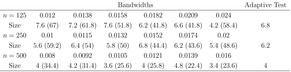
Table 5 reports the sizes of the proposed EL test as well as the single bandwidth
sets were chosen based on the same principle as outlined for the Vasicek models and
are reported in the table. The parameter estimation under these CIR models has the
same pattern of quality as the Vasicek model as reported in Table 2. We find that the
proposed test continued to have reasonable size for the three CIR models despite that
there were severe bias in the estimation ofκ. The size of the single bandwidth based
tests as well as the combined test were quite respectable for a sample size of 125. We
continue to see poor performance for the asymptotic test. It is interesting to see that
despite the quality of the parameter estimation still being poor for the CIR 2, the
severe size distortion observed earlier for Vasicek 2 was not present. Overall, the sizes
for the CIR models were better than the corresponding Vasicek models, which seemed
to suggest that the extra volatility offered by the CIR models “lubricates” the test
performance. Hong and Li’s test was also performed for the three CIR models and
are reported in Table 7. The performance was similar to that of the Vasicek models.
6.2. Power evaluation
To gain information on the power of the proposed test, we carried out simulation
that tested for the Vasicek model while the real process was the CIR 0 as in Pritsker’s
power evaluation of A¨ıt-Sahalia’s test:
dXt =κ(α−Xt)dt+σ
XtdBt, (6.2)
where κ = 0.89218, α = 0.09045 and σ2 = 0.032742. The region S was obtained by
rotating [0.015,0.25] ×[−0.015,0.015] 45 degrees anti-clock wise. The average CV
bandwidths based on 500 simulations were 0.0202 (the standard error of 0.0045) for
n= 125, 0.016991 (0.00278) for n = 250 and 0.014651 (0.00203) for n= 500.
Table 7 reports the power of the EL test and the single bandwidth based tests, as
well as the bandwidth sets used in the simulation. We find the tests had quite good
the power of the test tends to be larger than the maximum of the single bandwidth
based tests. This indicates that it possess attractive power properties. Table 7 also
reports the power of the Hong and Li’s test. It is found that the proposed test had
better power for all the sample sizes considered.
7. Case studies. We apply the proposed test on the Federal fund rates between
January 1963 and December 1998 which has n = 432 observations. A¨ıt-Sahalia
(1999) uses this data set to demonstrate the performance of the maximum likelihood
estimation. We test for five popular one-factor diffusion models which have been
proposed to model the dynamics of interest rates:
dXt = κ(α−Xt)dt+σdBt, (7.1)
dXt = κ(α−Xt)dt+σ
XtdBt, (7.2)
dXt = Xt{κ−(σ2−κα)Xt}dt+σXt3/2dBt, (7.3)
dXt = κ(α−Xt)dt+σXtρdBt, (7.4)
dXt = (α−1Xt−1+α0+α1Xt+α2Xt2)dt+σX 3/2
t dBt. (7.5)
They are respectively the Ornstein-Uhlenbeck process (7.1) proposed by Vasicek
(1977), the CIR model (7.2), the inverse of the CIR process (7.3), the constant
elastic-ity of volatilelastic-ity (CEV) model (7.4) and the nonlinear drift model (7.5) of A¨ıt-Sahalia
(1996).
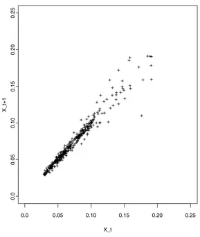
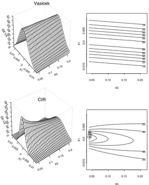
The data are displayed in Figure 1, which indicates a strong dependence as they
scattered around a narrow band around the 45-degree line. There was an increased
volatility when the rate was larger than 12%. The model-implied transitional densities
are displayed in Figure 2 using the MLEs given in A¨ıt-Sahalia (1999), which were used
in the formulation of the proposed test statistic. Figure 2 shows that the densities
implied by the Inverse CIR, the CEV and the nonlinear drift models were similar
The bandwidths prescribed by the Scott rule and the CV for the kernel estimation
were respectively href = 0.007616 and hcv = 0.00129. Plotting the density surfaces
indicated that a reasonable range forh was from 0.007 to 0.02, which offered a range
of smoothness from slightly undersmoothing to slightly oversmoothing. This led to
a bandwidth set consisting of 7 bandwidths with hmin = 0.007, hmax = 0.020 and
a= 0.8434.
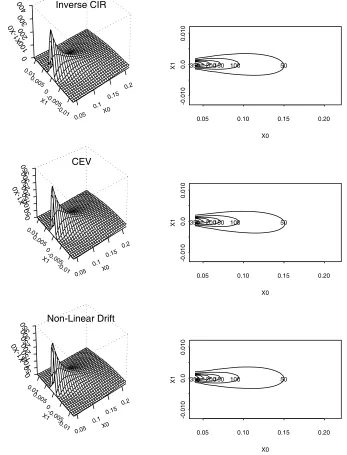
Kernel transitional density estimates and the smoothed model-implied transitional
densities for the five models are plotted in Figure 3 for h = 0.007. By comparing
Figure 2 with Figure 3, we notice the effect of kernel smoothing on these
model-implied densities.
In formulating the final test statistic Ln, we chose
N(h) = 1
n n
t=1
ℓ{p˜θ˜(Xt+1|Xt)}ω1(Xt, Xt+1), (7.6)
where ω1 is a uniform weight over a region by rotating [0.005,0.4]×[−0.03,0.03] 45
degree anticlock-wise. The region contains all the data pairs (Xt, Xt+1). As seen
from (7.6), N(h) is asymptotically equivalent to the statistic defined in (3.8) with
ω(x, y) =p(x, y)ω1(x, y), and has the same flavor with the test statistic of A¨ıt-Sahalia
(1996).
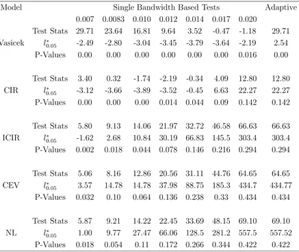
The p-values of the proposed tests as well as the tests based on single bandwidth
for each of the five diffusion models are reported in Table 8, which were obtained
based on 500 bootstrap resamples. It shows little empirical support for the Vasicek
model and quite weak support for the CIR. What is surprising is that there was quite
some empirical support for the inverse CIR, the CEV and the nonlinear drift models.
In particular, for CEV and the nonlinear drift models, the p-values of the single
bandwidth based tests were all quite supportive even for small bandwidths. Indeed,
by looking at Figure 3, we see quite noticeable agreement between the nonparametric
drift models.
8. Conclusion. The proposed test differs from the test of Hong and Li (2005)
in three aspects. The proposed test is based on a direct comparison between the
kernel estimate and the smoothed model-implied transitional density, whereas Hong
and Li’s test is an indirect comparison via data transformation. An advantage of the
direct approach is its robustness against poor quality parameter estimation which is
often the case for weak mean-reverting diffusion models. This is because both the
shape and the orientation of the transitional density are much less affected by the
poor quality parameter estimation. The second aspect is that Hong and Li’s test is
based on asymptotic normality and can be under the influence of slow convergence
discussed earlier although the transformed series is asymptotically independent. The
last aspect is that our proposed test is based on a set of bandwidths, which makes
the test robust against the choice of bandwidths.
The conclusion we draw from our studies is that the kernel method works
effec-tively for testing of diffusion models and is capable of modeling dependence induced
by a diffusion model. It is clear from the studies of Pritsker (1998) and this paper
that a proper implementation is vitally important. After all, the kernel method is
just an instrument for constructing nonparametric curve estimates. For a complex
task of testing a diffusion model, it will not work automatically by itself and requires
other procedures to make it work. However, what is working is the idea of comparing
the kernel estimate of a characteristic curve and the corresponding model-implied
curve of a diffusion model. This is the main idea of A¨ıt-Sahalia (1996). The role
of the kernel method is in translating the idea into some raw discrepancy measure.
Anything beyond it, for instance, the test statistic formulation and the choice of the
critical value should be the responsibilities of the other procedures.
computing assistance and a National University of Singapore Academic research grant
for generous support. The second author acknowledges support of an Australian
Research Council Discovery Grants Program.
Appendix. As the Lagrange multiplier λ(x, y) is implicitly dependent on h,
we need first to extend the convergence rate for a single h-based sup(x,y)∈Sλ(x, y)
conveyed in (3.6) uniformly over the bandwidth setH. To prove Theorem 1, we need
the following lemmas first.
Lemma A.1. Under Assumptions 1–4, maxh∈Hsup
(x,y)∈Sλ(x, y) =op{n−1/4log(n)}.
Proof: For anyδ >0
P
max
h∈Hn
sup
(x,y)∈S
hλ(x, y)≥δn−1/2log(n)
≤
h∈H
P
sup
(x,y)∈S
hλ(x, y)≥δn−1/2log(n)
.
As the number of bandwidths inH is finite, by checking the relevant derivations in Chen,
H¨ardle and Li (2002), it can be shown that
P
⎛
⎝
(x,y)∈S
hλ(x, y)≥δn−1/2log(n) ⎞
⎠→0
as n → ∞. This implies that maxh∈Hsup(x,y)∈Shλ(x, y) = op{δn−1/2log(n)}. Then the
lemma is established by noting thathmin, the smallest bandwidth in Hn, is of order n−γ1
whereγ1∈(0,1/4) as assumed in Assumption 1.
Before introducing the next lemma, we present some expansions for the EL test statistic
N(h). Let
˜
pθ(x, y) = ˜pθ(y|x)ˆπ(x) and p˜(x, y) =n−1 n+1
t=1
Kh(x−Xt) n+1
s=1
ws(y)p(Xs|Xt)
be kernel smooths of the parametric and real underlying joint densitiespθ(x, y) andp(x, y)
respectively. Due to the relationship between transitional and joint densities, from (3.8)
N(h) = (nh2)
{pˆ(x, y)−p˜θ˜(x, y)}2
R2(K)p(x, y) ω(x, y)dxdy+ ˜Op{h
2+ (nh2)−1/2log3(n)}
= (nh2)R−2(K)
{pˆ(x, y)−p˜(x, y)}2
p(x, y) +
2{pˆ(x, y)−p˜(x, y)}{p˜(x, y)−p˜θ˜(x, y)}
+ {p˜(x, y)−p˜θ˜(x, y)}
2
p(x, y)
ω(x, y)dxdy+ ˜Op{h2+ (nh2)−1/2log3(n)}
=: N1(h) +N2 ˜θ(h) +N3 ˜θ(h) + ˜Op{h2+ (nh2)−1/2log3(n)} (A.1)
Here and throughout the proofs, ˜o(δn) and ˜O(δn) denote stochastic quantities which are
respectivelyo(δn) and O(δn) uniformly overS for a non-negative sequence{δn}.
Using Assumptions 3.3 and 3.4, we have Nlθ˜(h) = Nlθ∗(h) + ˜Op(n−1/2) where θ∗ =θ0
underH0 andθ1 under H1. Thus,
N(h) = N1(h) +N2θ∗(h) +N3θ∗(h) + ˜Op{h2+ (nh2)−1/2log3(n)}
We start with some lemmas on ˆp(x, y), ˜p(x, y) and ˜pθ(x, y). Let K(2) be the
con-volution of K, M K(2)(t) =
uK(u)K(t+u)du and p3(x, y, z) be the joint density of
(Xt, Xt+1, Xt+2).
Lemma A.2. Under Assumptions 1–4, we have,
Cov{pˆ(s1, t1),pˆ(s1, t1)} =
K(2)s2−s1
h
K(2)s2−s1
h
p(s1, t1)
nh2
− M K
(2)s2−s1
h
∂p(s1,t1)
∂x +M K(2)
t2−t1
nh
∂p(s1,t1)
∂y
nh
+ p3(s1, t1, t2)K
(2)s2−t1
h
+p3(s2, t2, t1)K(2)
s1−t2
h
nh
+ o{(nh)−1}.
Proof: LetZt(s, t) =Kh(s−Xt)Kh(t−Xt+1) so that ˆp(s, t) =n−1n
t=1Zt(s, t) and
Cov{pˆ(s1, t1),pˆ(s1, t1)} = n−1Cov{Z1(s1, t1), Z1(s2, t2)} (A.2)
+ 1
n−1[Cov{Z1(s1, t1), Z2(s2, t2)}+ Cov{Z2(s1, t1), Z1(s2, t2)}]
+ Qn,
whereQn=n−1nl=2−1(1−ln−1)[Cov{Z1(s1, t1), Zl+1(s2, t2)}+Cov{Zl+1(s1, t1), Z1(s2, t2)}].
Standard derivations show that
Cov{Z1(s1, t1), Z1(s2, t2)} =
K(2)s2−s1
h
K(2)s2−s1
h
p(s1, t1)
h2
− M K
(2)s2−s1
h
∂p(s1,t1)
∂x +M K(2)
t2−t1
h
∂p(s1,t1)
∂y
nh + ˜O(1)
Cov{Z1(s1, t1), Z2(s2, t2)} =
p3(s1, t1, t2)K(2)s2−ht1
Apply Davydov inequality forα-mixing sequences via the same route of Fan and Gijbles
(1996, P.251) thatQn= ˜o{(nh)−1). This together with (A.2) - (A.3) lead prove the lemma.
That α-mixing leads to Qn = ˜o{(nh)−1), the pre-whitening effect of smoothing
band-width, is a fact that we will use repeatedly without further mentioning.
Lemma A.3. Suppose that Assumptions 1–4 hold. Let∆θ(x, y) ={pθ(y|x)−p(y|x)}π(x). Then
E{p˜θ(x, y)−pˆ(x, y)} = ∆θ(x, y) + 12h2σ2K{ ∂ 2 ∂x2 + ∂
2
∂y2}∆θ(x, y) + ˜O(h3), (A.4)
E{p˜θ(x, y)−p˜(x, y)} = ∆θ(x, y) + 12h2σ2K{ ∂ 2 ∂x2 + ∂
2
∂y2}∆θ(x, y) + ˜O(h3), (A.5)
Cov{p˜(s1, t1),p˜(s2, t2)} =
K(2)t2−t1
h
p(s1, t1)p(s2, t1)
nhπ(t2)
+ ˜o{(nh)−1}. (A.6)
Proof: As ˜pθ(x, y) =n−1n+1
t=1 Kh(x−Xt)
n+1
s=1 ws(y)pθ(Xs|Xt), from the bias of the
local linear regression (Fan and Gijbels, 1996) and kernel density estimators, and that the
transitional density has uniformly bounded thrid derivatives in Assumption 3,
E{p˜θ(x, y)} = E{n−1 n+1
t=1
Kh(x−Xt){pθ(y|Xt) +12h2σK2 ∂ 2pθ(y
|Xt)
∂y2 + ˜Op(h3)}
= pθ(y|x)π(x) +12h2σK2{ ∂ 2 ∂x2 + ∂
2
∂y2}pθ(y|x)π(x) + ˜O(h3).
Then employing the same kind of derivation onE{pˆ(x, y)}, we readily establish (A.4).
For the purpose of deriving (A.6), we note the following expansion for ˜p(x, y) based on
the notion of equivalent kernel for local linear estimator (Fan and Gijbels, 1996):
˜
p(x, y) = n−1Kh(x−Xt) n+1
s=1
ws(y)pθ(Xs|Xt)
= n−1Kh(x−Xt) n+1
s=1
π−1(y)Kh(y−Xs)pθ(Xs|Xt){1 + ˜op(h)}
= π(x)π−1(y)
n+1
s=1
π−1(y)Kh(y−Xs)pθ(Xs|x){1 + ˜op(h)}. (A.7)
Then derivations similar to those used in Lemma A.2 readily establish (A.6).
Lemma A.4. Under Assumptions 1–4, we have
Cov{pˆ(s1, t1),p˜(s2, t2)} =
p(s1, t1)
nhπ(t2)
K(2)
t2−s1
h
p(s2, s1) +K(2)
t2−s1
h
p(s2, s1)
Proof: From (A.7),
Cov{pˆ(s1, t1),p˜(s2, t2)}
= π(s2)
nπ(t2)
Cov{Kh(s1−X1)Kh(t1−X2), Kh(t2−X1)p(X1|s2)}
+ Cov{Kh(s1−X1)Kh(t1−X2), Kh(t2−X2)p(X2|s2)}
{1 + ˜o(1)}
= π(s2)
nhπ(t2){
K(2)
t2−s1
h
p(s1|s2)p(s1, t1) +K(2)
t2−t1
h
p(t1|s2)p(s1, t1)}{1 + ˜o(1)}
which then leads to the statement of the lemma. .
Lemma A.5. IfH0 is true, then N2θ∗(h) =N3θ∗(h) = 0 for allh∈ H.
Proof: Under H0, p(y|x) = pθ
0(y|x) and θ∗ = θ0. Hence, ˜p(x, y) −p˜θ∗(x, y) =
n−1
Kh(x−Xt)ws(y){p(Xs|Xt)−pθ0(Xs|Xt)}= 0. This completes the proof.
Lemma A.6. Suppose that Assumptions 1–4 hold. If H1 is true, then
N2θ∗(h) = O˜p{(nh2)−1/2log(n)} ×
∆θ1(x, y)
p(x, y) ω(x, y)dxdy and (A.8)
N3θ∗(h) = (nh2)R−2(K)
∆2(x, y)
p(x, y) ω(x, y)dxdy{1 + ˜op(1)} (A.9)
uniformly over the bandwidth set H.
Proof: UnderH1,θ∗ =θ1. Standard derivation as those in Lemma A.3 show that
˜
p(x, y)−p˜θ1(x, y) = p˜(x, y)−E{p˜(x, y)}+E{p˜(x, y)} −E{p˜θ1(x, y)}
+ E{p˜θ1(x, y)} −p˜θ1(x, y)
= −∆θ1(x, y) + ˜Op{(nh)−
1/2) log(n) +h2
}. (A.10)
This and the fact that ˆp(x, y)−p˜(x, y) = ˜O{(nh2)−1/2log(n) +h3}= ˜O{(nh2)−1/2log(n)}
lead to (A.8). And (A.9) can be argued similarly using (A.10).
Let us now study the leading term N1(h). From (A.1) and by hiding the variables of
integrations,
N1(h) =
(nh2)
R2(K)
{pˆ−p˜}2
R2(K)pω
= (nh
2)
R2(K)
{pˆ−Epˆ}2
p +
{Ep˜−p˜}2
p +
{Epˆ−Ep˜}2
+ 2{pˆ−Epˆ}{Epˆ−Ep˜}
p +
2{pˆ−Epˆ}{Ep˜−p˜}
p +
2{Epˆ−Ep˜}{Ep˜−p˜}
p ω =: 6 j=1
N1j(h) (A.11)
We are to show in the following lemmas that N11(h) dominates N1(h) and N1j(h) for
j≥2 are all negligible exceptN12(h) which contributes to the mean ofN1(h) in the second
order.
Lemma A.7. Under Assumptions 1–4, then uniformly with respect to H
h−1E{N11(h)−1} = o(1), (A.12)
Var{h−1N11(h)} =
2K(4)(0)
R4(K)
ω2(x, y)dxdy+o(1), (A.13)
Cov{h−11N11(h1), h−21N11(h2)} =
2ν(h1/h2)
R4(K)
ω2(x, y)dxdy+o(1). (A.14)
Proof: From Lemma A.1 and note thatM K(2)(0) = 0
E{N11(h)} =
nh2
R2(K)
V ar
{pˆ(x, y)}
p(x, y) ω(x, y)dxdy
= 1
R2(K)
K(2)(0)2+ 2hK(2)
y−x h
p3(x, y, y)
p(x, y)
× ω(x, y)dxdy{1 +o(1)}= 1 +O(h2), (A.15)
which leads to (A.12). To derive (A.13), let
ˆ
Zn(s, t) = (nh2)1/2
ˆ
p(s, t)−Epˆ(s, t)
R(K)p1/2(x, t) .
It may be shown from the fact that K is bounded and other regularity condition
as-sumed that E{|Zˆn(s1, t1)|2+ǫ|Zˆn(s2, t2)|2+ǫ} ≤ M for some positive ǫ and M. And hence
{Zˆn(s, t)}n≥1 and {Zˆn2(s1, t1) ˆZn2(s1, t1)}n≥1 are uniformly integrable respectively. Also,
ˆ
Zn(s1, t1),Zˆn(s2, t2)
T d
→ (Z(s1, t1), Z(s2, t2))T which is a bivariate normal random
vari-able with mean zero and a covariance matrix
Σ = ⎛
⎜ ⎝
1 g{(s1, t1),(s2, t2)}
g{(s1, t1),(s2, t2)} 1
⎞
whereg{(s1, t1),(s2, t2)}=K(2)
s2−s1
h
K(2)t2−t1
h
p1/2(s1,t1)
R(K)p1/2(s
2,t2). Hence,
Var{N11(h)} =
Cov{Zˆn2(s1, s2),Zˆn2(s2, t2)}ω(s1, t1)ω(s2, t2)ds1dt1ds2dt2
=
Cov{Z2(s1, s2), Z2(s2, t2)}ω(s1, t1)ω(s2, t2)ds1dt1ds2dt2
= 2
Cov2{Z(s1, s2), Z(s2, t2)}ω(s1, t1)ω(s2, t2)ds1dt1ds2dt2
= 2
R4(K)
{K(2)
s2−s1
h
K(2)
t2−t1
h
}2R2(pK(s)1p, t(s1) 2, t2) ×ω(s1, t1)ω(s2, t2)ds1dt1ds2dt2
= 2h
2K(4)(0)
R4(K)
ω2(s, t)π−2(t)dsdt (A.16)
the second to fourth equations are valid up to a factor {1 +o(1)}. In the third equation
above, we use a fact regarding the fouth product moments of normal random variables.
Combining (A.15) and (A.16), (A.12) and (A.13) are derived. It is trivial to check that it
is valid uniformly for allh∈ H.
The proof for (A.14) follows that for (A.13).
Lemma A.8. Under Assumptions 1–4, then uniformly with respect to h∈ H
h−1N12(h) =
1
R(K)
p(x, y)
π(y) ω(x, y)dxdy+op(1), (A.17)
h−1N1j(h) = op(1). for j≥3 (A.18)
Proof: From (A.6) and the fact thatK(2)(0) =R(K),
E{N12(h)} =
(nh2)
R2(K)
Var
{p˜}
p ω
= h
R(K)
p(x, y)
π(y) ω(x, y)dxdy{1 + ˜o(1)}. (A.19)
Let ˜Zn(s, t) = (nh)1/2 ˜p(s,t)R1/2(K)p(x,t)−Ep(s,t)˜ . Using the same approach that derives (A.16) and from
Lemma A.2
Var{N12(h)} =
h2
R2(K)
Cov{Z˜n2(s1, s2),Z˜n2(s2, t2)}ω(s1, t1)ω(s2, t2)ds1dt1ds2dt2
= 2h
2
R4(K)
{K(2)
t2−t1
h
}2π−2(t2)ω(s2, t2)ds1dt1ds2dt2
= 2h
4K(4)(0)
R4(K)
up to a factor{1+ ˜o(1)}. Combining (A.19) and (A.20), (A.17) is derived. It can be checked
that it is valid uniformly for allh∈ H.
As {Epˆ(x, y)−Ep˜(x, y)}2= ˜O(h6) and h=o(n−1/7) for allh∈ H, we have (nh2)h6 =
op(h) uniformly for allh∈ H and hence (A.15) forj = 2.
Obviously E{N14(h)} = 0. Use the same method for Var{N12(h)} and from Lemmas
A.1 and A.2,
Var{N14(h)} =
4(nh2)2
R4(K)
E{pˆ−p˜}(s1, t1)E{pˆ−p˜}(s2, t2)Cov{pˆ(s1, t1),ˆp(s2, t2)}
p(s1, t1)p(s2, t2) ×w(s1, t1)w(s2, t2)ds1dt1ds2dt2
AsE{pˆ−p˜}(s1, t1)E{pˆ−p˜}(s2, t2) =O(h6) and the integral over the covariance produces
a h2 in addition to (nh2)−1. Thus, V ar{N14(h)} = O{(nh2)h6h2} = o(h2) uniformly for
all h ∈ H. This means that N14 = op(h) uniformly for all h ∈ H. Using exactly the
same derivation, but employing Lemma A.3 instead of Lemma A.1, we have N16 = op(h)
uniformly for allh∈ H.
It remians to studyN15(h). From Lemma A.3,
E{N15(h)} = −
2(nh2)
R2(K)
Cov{pˆ(x, y),˜p(x, y)}
p(x, y) ω(x, y)dxdy
= − 4h
R2(K)
K(2)y−x
h
p(x, y)
π(y) ω(x, y)dxdy
= − 4h
2
R2(K)
K(2)(u)du
π(y)ω(y, y)dy{1 + ˜o(1)}.
using Assumption 1(iv). It may be shown using the same method that derives (A.20) that
Var{N15(h)}=o(h2) and hence N15(h) =op(h).
Let L(h) = C(K)h1 {N(h)−1} and β= C(K)R(K)1 p(x,y)
π(y) ω(x, y)dxdy. In view of
Lem-mas A.5, A.7 and A.8, we have underH0, uniformly with respect toH,
L(h) = 1
C(K)h{N11(h)−1}+β+op(1) (A.21)
Define L1(h) = C(K)h1 {N11(h)−1}.
Lemma A.9. Under Assumptions 1–4 and H0, asn→ ∞,
Proof: According to the Cram´er–Wold device, in order to prove Lemma A.9, it suffices
to show that
k
i=1
ciL1(hi)→d NJ(0, cτΣJc) (A.22)
for an arbitrary vector of constants c = (c1,· · ·, ck)τ. Without loss of generality, we will
consider only the proof for the case ofk= 2. To apply Lemma A.1 of Gao and King (2003),
we introduce the following notation. Fori= 1,2, definedi = √ci2hi and ξt= (Xt, Xt+1),
ǫti(x, y) = K
x−Xt
hi
K
y−Xt+1
hi −E K
x−Xt
hi
K
y−Xt+1
hi
,
φi(ξs, ξt) =
1
nh2 i
ǫsi(x, y)ǫti(x, y)
p(x, y)R2(K) ω(x, y)dxdy,
φst = φ(ξs, ξt) = 2
i=1
diφi(ξs, ξt) and L1(h1, h2) = T
t=2 t−1
s=1
φst. (A.23)
It is noted that for any givens, t≥1 and fixed x and y,E[φ(x, ξt)] = E[φ(ξs, y)] = 0.
Since the asymptotic variancecτΣ
Jcis a non–random quadratic form depending neither on
h nor onn, in order to apply their Lemma A.1, it suffices to verify
max{Mn, Nn}h1−2 →0 asn→ ∞, (A.24)
where
Mn = max
n2M
1 1+δ n1 , n2M
1 2(1+δ) n51 , n2M
1 2(1+δ) n52 , n2M
1 2 n6
Nn = max
n32M 1 2(1+δ) n21 , n
3 2M
1 2(1+δ) n22 , n
3 2M
1 2 n3, n
3 2M
1 2(1+δ) n4 , n
3 2M 1 1+δ n7 , in which
Mn1 = max
1≤i<j<k≤nmax
E|φikψjk|1+δ,
|φikθjk|1+δdP(ξi)dP(ξj, ξk)
,
Mn21 = max
1≤i<j<k≤nmax
E|φikφjk|2(1+δ),
|φikφjk|2(1+δ)dP(ξi)dP(ξj, ξk)
,
Mn22 = max
1≤i<j<k≤nmax
|φikφjk|2(1+δ)dP(ξi, ξj)dP(ξk),
|φikφjk|2(1+δ)dP(ξi)dP(ξj)dP(ξk)
,
Mn3 = max
1≤i<j<k≤nE|φikφjk|
2, M
n4= max
1< i, j, k≤2n
i, j, kdifferent
max
P
|φ1iφjk|2(1+δ)dP
where the maximization overP in the equation forMn4 is taken over the four probability
measuresP(ξ1, ξi, ξj, ξk),P(ξ1)P(ξi, ξj, ξk),P(ξ1)P(ξi1)P(ξi2, ξi3), andP(ξ1)P(ξi)P(ξj)P(ξk),
where (i1, i2, i3) is the permutation of (i, j, k) in ascending order;
Mn51 = max
1≤i<j<k≤nmax
E
φikφjkφikφjkdP(ξi)
2(1+δ) ,
Mn52 = max
1≤i<j<k≤nmax
φikφjkφikφjkdP(ξi)
2(1+δ)
dP(ξj)dP(ξk) ,
Mn6 = max 1≤i<j<k≤nE
φikφjkdP(ξi)
2
, Mn7= max 1≤i<j<nE
|φij|1+δ
.
Due to the fact thatφst is only a linear combination of φ1(Xs, Xt) andφ2(Xs, Xt), in
order to verify the above conditions, it suffices to verify that each φi(Xs, Xt) satisfies the
conditions. In the following, we will only deal with the case of i = 1, as the other case
follows similarly.
Without any confusion, we replace h1 by h for simplicity. To verify the Mn part of
(A.24), we verify only
lim
n→∞n
2h−2M1+1δ
n1 = 0. (A.25)
Let q(x, y) =ω(x, y)p−1(x, y) and
ψij =
1
nh2
K((x−Xi)/h)K((y−Xi+1)/h)K((x−Xj)/h)K((y−Xj+1)/h)q(x, y)dxdy
for 1≤i < j < k≤n. Direct calculation implies
ψikψjk = (nh2)−2
· · ·
K
x−Xi
h
K
y−Xi+1
h
K
x−Xk
h
K
y−Xk+1
h
q(x, y)
× K
u−Xj
h
K
v−Xj+1
h
K
u−Xk
h
K
v−Xk+1
h
q(u, v)dxdydudv
= bijk+δijk,
whereδijk =ψikψjk−bijk and
bijk = n−2q(Xi, Xi+1)q(Xj, Xj+1)
× K(2)
Xi−Xk
h
K(2)
Xj−Xk
h
K(2)
Xi+1−Xk+1
h
K(2)
Xj+1−Xk+1
h
,
For any given 1< ζ <2 and nsufficiently large, we may show that
Mn11 = E
|ψijψik|ζ
≤2E|bijk|ζ
+E|δijk|ζ
= 2E|bijk|ζ
(1 +o(1))
= n−2ζ
|q(x, y)q(u, v)|ζ K(2)
x−z h
K(2)
u−z h ζ × K(2)
y−w h
K(2)
v−w h ζ
p(x, y, u, v, z, w)dxdydudvdzdw
= C1n−2ζh4 (A.26)
where p(x, y, u, v, z, w) denotes the joint density of (Xi, Xi+1, Xj, Xj+1, Xk, Xk+1) and C1
is a constant. Thus, asn→ ∞
n2h−2M
1 1+δ
n11 =Cn2h−1
n−2ζh21/ζ=h2(2−ζζ) →0. (A.27)
Hence, (A.27) shows that (A.25) holds for the first part ofMn1. The proof for the second
part ofMn1 follows similarly. As for (A.26), we have that asn→ ∞
Mn3 = E|ψikψjk|2= (nh2)−4h8
|q(x, y)q(u, v)|2 K(2)
x−z h
K(2)
y−z h 2 × K(2)
u−w h
K(2)
v−w h 2
p(x, y, z, u, v, w)dxdydzdudvdw
= C1n−4h4,
whereC2 is a constant. This implies that asn→ ∞
n3/2h−2M
1 2
n3 =Cn−1/2 →0. (A.28)
Thus, (A.28) now shows that (A.24) holds forMn3. It follows from the structure of {ψij}
that (A.24) holds automatically forMn51,Mn52andMn6. We now start to prove that (A.25)
holds forMn21. For some 0< δ <1 and 1≤i < j < k≤n, letMn21=E
!
|ψikψjk|2(1+δ)
" .
Similarly to (A.26) and (A.27), we obtain that asn→ ∞
n3/2h−2M
1 2(1+δ)
n21 →0. (A.29)
This finally completes the proof of (A.25) forMn21and thus (A.25) holds for the first part of
{φ1(Xs, Xt)}. Similarly, one can show that (A.24) holds for the other parts of{φ1(Xs, Xt)}.
Proof of Theorem 1: From (A.21) and Lemma A.9, we have under H0
(L(h1),· · ·, L(hJ))→d NJ(β1J,ΣJ).
LetZ = (Z1,· · ·, Zk)T d∼NJ(β1k,ΣJ). By the mapping theorem, under H0,
Ln= max
h∈HL(h)
d →max
1≤kJZk. (A.30)
Hence the theorm is established. .
Let l0α be the upper-α quantile of max1≤ikZi. As the distribution of NJ(β1k,ΣJ) is
free ofn, so is that of max1≤ikZi. And hence l0α is a fixed quantity with respect ton.
The following lemmas are required for the proof of Theorem 2.
Lemma A.10. Under Assumptions 1–4 and H1, for any fixed real value x, as n→ ∞,
P(Ln≥x) →1.
Proof: Let A = R−2(K) ∆2(x,y)
p(x,y) ω(x, y)dxdy. From Lemmas A.6 and A.7, under
H1, (nh2)−1N(h) =A+op(1) uniformly with respect to H. Hence, (nh)−1L(h) = C(K)A +
op(1) for all h ∈ H. Hence, for some i ∈ {1, . . ., k}, P(Ln < x) ≤ P{L(hi) < x} =
P{(nh)−1L(hi)<(nh)−1x}. As (nh)−1L(hi) p
→ C(K)A >0 and (nh)−1x→0, hence P(Ln<
x)→0.
We now turns to the bootstrap EL test statisticN∗(h), which is a version ofN(h) based
on{Xt∗}n+1t=1 generated according to the parametric transitional density pθ˜. Let ˆp(x, y) and
˜
p∗
θ(x, y) are the bootstrap versions of ˆp(x, y) and ˜p(x, y) respectively, and ˜θ∗be the maximum
likelihood estimate based the bootstrap sample. Then, the following analogue expansion to
(A.2) is valid forN∗(h)
N∗(h) = (nh2)
{pˆ∗(x, y)−p˜∗
˜
θ∗(x, y)}
2
R2(K)p ˜ θ(x, y)
ω(x, y)dxdy+ ˜op{h}
= N1∗(h) +N∗
2 ˜θ(h) +N3 ˜∗θ(h) + ˜op(h)
where Nj∗(h) for j = 1,2 and 3 are the bootstrap version of Nj(h) resepctively. As the
bootstrap resample is generated according topθ˜, the same arguments which lead to Lemma
5 mean that N2∗(h) =N3∗(h) = 0. Thus, N∗(h) =N1∗(h) + ˜op(1) where
N1∗(h) = (nh2)
{pˆ∗(x, y)−p˜∗(x, y)}2
R2(K)p ˜ θ(x, y)
And similar lemmas to Lemmas A.7 and A.8 can be established to studyN1j∗(h) which are
the boostrap version ofN∗
1j(h) respectively.
Let L∗(h) = C(K)h1 {N(h)−1} and ˆβ = C(K)R(K)1 pθ˜(x,y)
πθ˜(y) ω(x, y)dxdy.
Lemma A.11. Under Assumptions 1–4, asn→ ∞, given{Xt}n+1
t=1,
(L∗(h1),· · ·, L∗(hk))→d NJ( ˆβ1J,ΣJ).
Proof: The proof follows that of Theorem 1 with the real underlying transitional density
pθ˜ to replacep in the proof of Theorem 1.
Let l∗α be the upper-α conditional quantile ofL∗n= maxh∈HL∗(h) given{Xt}n+1t=1.
Proof of Theorem 2: (i) Let ˆZ = ( ˆZ1, . . .,Zˆk)T such that its conditional distribution given{Xt}n+1t=1 isNJ( ˆβ1J,ΣJ) andl∗0α be the upper-α conditional quantile of max1≤i≤kZˆi.
As ˜θ=θ+Op(n−1/2) as assumed in Assumption 5 (i), ˆβ=β+Op(n−1/2). This means that
max1≤i≤kZˆi = max1≤i≤kZi+op(1). Therefore,l0α∗ =l0α+op(1). From Lemma A.11, we
have via the mapping theorem again, limn→∞P{L∗n≥l0α∗ |{Xt}n+1t=1}=α. Therefore,
l∗α=l0α+op(1). (A.31)
AsLn→d max1≤i≤kZi, by Slutsky theorem,
P(Ln≥l∗α) =P(Ln+op(1)≥l0α)→P( max
1≤i≤kZi≥l0α) =α
which completes the part (i) of Theorem 2. The part (ii) of Theorem 2 is a direct
conse-quence of Lemma A.9 and (A.31).
REFERENCES
A¨ıt-Sahalia, Y. (1996). Testing continuous-time models of the spot interest rate. Review of Financial
Studies 9 385–426.
A¨ıt-Sahalia, Y. (1999). Transition densities for interest rate and other nonlinear diffusions. Journal
of Finance54 1361–1395.
A¨ıt-Sahalia, Y. (2002). Maximum likelihood estimation of discretely sampled diffusions: a closed–
form approximation approach. Econometrica70223–262.
A¨ıt-Sahalia, Y., Bickel, P. and Stoker, T. (2001). Goodness–of–fit tests for regression using kernel