http://dx.doi.org/10.4236/wjet.2015.32008
Performance Study of PID Controller and
LQR Technique for Inverted Pendulum
Akhil Jose, Clint Augustine, Shinu Mohanan Malola, Keerthi Chacko
Department of Electronics and Instrumentation Engineering, Vimal Jyothi Engineering College, Kannur, India Email: [email protected], [email protected]
Received 8 April 2015; accepted 19 May 2015; published 22 May 2015
Copyright © 2015 by authors and Scientific Research Publishing Inc.
This work is licensed under the Creative Commons Attribution International License (CC BY). http://creativecommons.org/licenses/by/4.0/
Abstract
The inverted pendulum is a classic problem in dynamics and control theory and is widely used as a benchmark for testing control algorithms. It is unstable without control. The process is non linear and unstable with one input signal and several output signals. It is hence obvious that feedback of the state of the pendulum is needed to stabilize the pendulum. The aim of the study is to stabilize the pendulum such that the position of the carriage on the track is controlled quickly and accu-rately. The problem involves an arm, able to move horizontally in angular motion, and a pendulum, hinged to the arm at the bottom of its length such that the pendulum can move in the same plane as the arm. The conventional PID controller can be used for virtually any process condition. This makes elimination the offset of the proportional mode possible and still provides fast response. In this paper, we have modelled the system and studied conventional controller and LQR controller. It is observed that the LQR method works better compared to conventional controller.
Keywords
Control System, LQR Technique, Conventional Controller, Inverted Pendulum
1. Introduction
Generally, all systems are initially checked with conventional controllers including P, PI, and PID [1] since it is easy to develop and implement. Various methods are available for tuning these controllers. If the response is not satisfactory advanced, controllers are considered. When the system is non-linear and with significant delay, conventional controllers cannot give a satisfactory result [2]. LQR controller is a suitable alternative in such case. It can deal with non-linear systems efficiently. Pole placement methods like Ackerman’s formula are very popular in designing the state feedback gain K and hence to place the poles in desired locations [3]-[5]. But in these methods, we need to specify the desired poles to seek the SVFB gain. Also these methods are only appli-cable for single input systems. However, it is very inconvenient to specify all the closed loop poles and we would like to have a technique that works for many numbers of inputs. Due to these constrains, we make use of the theory of optimal control for the design of a better controller. Optimal controllers are designed in sense of using the least required control effort to maintain equilibrium [6]. Optimal control principle is inspired from naturally occurring systems which are optimal.
In Section 2, the problem is identified and defined. In Section 3, a detailed description about the experimental setup and system modelling is given. Section 4 describes about the designing of PID controller and LQR con-troller for the system. In Section 5, the simulation results are compared and Section 6 contains conclusion.
2. Problem Definition
The problem of controlling an inverted pendulum is to balance the pendulum in its upright position by moving the arm in opposite direction. The control output is limited by several constraints like the speed of motor con-trolling the arm. In this study, simulation of control in inverted pendulum system has been carried out using MATLAB and Simulink software.
3. Experimental Setup and Description
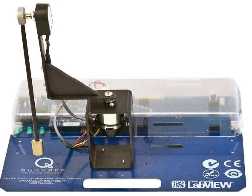
AQuanser rotary inverted pendulum which we used for modelling is shown in Figure 1. The inverted pendulum is hinged to its arm.
The horizontal movement of the arm and the pendulum vertical position angle are measured by optical en-coder. The encoders produce 4096 pulses for revolution, which gives a very reasonable precision in measure-ment. The arm motion is actuated by a DC motor. The DC motor is controlling the rotary motion of the arm. Encoder is used to feedback the angular position of the pendulum to servo electronics to generate actuating sig-nal. The controller circuits provide the controlling signal which then drives the arm through the servomotor. Ro-tary motion of the arm applies moments on the inverted pendulum and keeps the pendulum upright.
[image:2.595.188.446.506.707.2]Figure 2. Diagram model for the system.
The kinetic and potential energies are given by the following equations:
cos
pot p p
E =M gl α (1)
(
)
2(
)
21 1
cos sin
2 2
kinP p p p p
E = M θl α + M αl α (2)
( )
21
2 kinArm p
E = J θ (3)
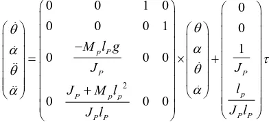
where Jpand Mp are arm inertia and pendulum mass respectively. Applying Lagrangian formula for the
equa-tions the state space model is obtained
2
0 0 1 0 0
0 0 0 1 0
1
0 0 0
0 0 0
p P
P P
p
P p p
P P P P
M l g
J J
l
J M l
J l J l θ θ α α τ θ θ α α × − = + + (4)
τ is the torque of the motor. Known constant values are given in the table 1 shown below.
Substituting the known values in the equations we obtain the state space model of the system. The new state description of the system with voltage as input is given below:
0 0 1 0 0
0 0 0 1 0
0 22.37 0.2982 0 8.9578
0 36.2 0.0765 0 2.2980
V θ θ α α θ θ α α × = + − − (5)
The transfer function model of the system obtained is given as:
( )
4 2 3 22.298 0.000187 2.8 15
0.298 36.2 9.083
s s e
G s
s s s s
− − −
=
+ − − (6)
4. Controller Design
MATLAB and Simulink is discussed in this section
4.1. PID controller Design
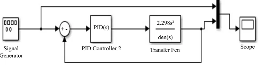
PID controller is the most widely used controllers for industrial applications [8]. PID controller design schemes are easy and robust in nature [9]. Defining “u” as the controller output, the final PID algorithm is of the form:
( )
0( )
d( )
d
d
p i p
t
u K e t K e K e t
t τ τ
= +
∫
+where Kp, Ki, Kd are proportional, integral and derivative gains respectively which are the tuning parameters
used to design a PID controller. We used the transfer function model of the system to design a PID controller in Simulink. The Simulink model of the PID controller is given in Figure 3.
The values of tuning parameters Kp, Ki, and Kd are 516.35, 431.787 and 61.63 respectively.
4.2. LQR Controller Design
In this section, an LQR controller is developed for the inverted pendulum system. The LQR method uses the state feedback approach for controller design. As discussed, the system is expressed in state variable form as
x= Ax+Bu. We assume that all the states are measurable. The state variable feedback control can be found from the expression u= −Kx+v.
Using this control closed loop system becomes x=
(
A BK x−)
+Bv=A xc +Bv with Ac the closed loop plantmatrix and v(t) the new command input. C and D matrices are not used in the SVFB design. To design an optimal SVFB we may define a performance index.
T T
0
1
d . 2
J x Qx u Ru t
∞
=
∫
+Substituting the SVFB we yields
(
)
T T
0
1
d 2
J x Q K RK x t
∞
=
∫
+We assume v(t) as zero as our only concern is internal stability of the system. The objective is to select the K that minimizes the performance index J. Q and R must be selected to be positive semi-definite and positive defi-nite in order to minimize J. The feedback gain matrix K in LOR is solved using the equation
K
=
R B P
−1 T . To seek P we make use of a very important formula in modern control theory known as Algebraic Riccati Equation (ARE).T 1 T
0
A P+PA Q+ −PBR B P− =
The design procedure for finding the feedback gain K for LQR can be formulated to 3 simple steps:
• Select the design parameter matrices Q and R.
• Find P by solving the ARE.
[image:4.595.94.536.583.700.2]• Find the state feedback matrix K using
K
=
R B P
−1 T.
The LQR guarantees pole placement and stability to the closed loop system as long as two LQR theorems [References] hold:
LQR theorem 1
Let the system (A, B) be reachable. Let R be positive definite and Q be positive definite. Then the closed loopsystem (A-BK) is asymptotically stable.
LQR theorem 2
Let the system (A, B) be stabilizable. Let R be positive definite, Q be positive semi definite, and
(
A, Q)
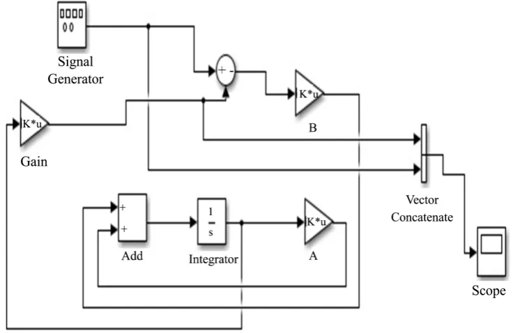
be observable. Then the closed loop system (A-BK) is asymptotically stable. The simulink model for state feedback controller is shown in Figure 4.The SVFB gain K is found using lqr command in Matlab and this gain is given in the Simulink model to ob-tain the outout.
The value of Q matrix which gave the best pole placement was [100 0 0 0; 0 1 0 0; 0 0 200 0; 0 0 0 1] and R matrix was selected as [1].
The value of K derived is [−10.0000 719.0337 −17.8791 129.8297].
5. Results and Discussion
The PID and LQR controller performance for the system is simulated MATLAB Simulink. Q and R values are selected based on fine tuning by trial and error method. Responses of both the systems are studied with a square wave as input. The results of both the controllers are discussed in this section.
5.1. PID Controller Response
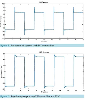
The response of the system with PID controller is shown in Figure 5. PID controller tuning for the proposed system model is showing only a very narrow region of stability. When the gains are increased, the system is set-tled fast but the overshoot is very high. When we reduce the overshoot by reducing the gain, the settling time has to pay the price. Figure 5 shows a reasonably good response obtained by tuning the PID controller.
5.2. LQR Response
The LQR controller gives a much stable and robust response for the system. The response of the system with LQR controller is given in Figure 6.
Figure 5.Response of system with PID controller.
Figure 6. Regulatory response of PI controller and FLC.
There is a considerable reduction in overshoot and settling time with the LQR controller. The response is more stable and robust.
References
[1] Lozano, R., Fantoni, I. and Block, D.J. (2000) Stabilization of the Inverted Pendulum around Its Homoclinic Orbit. Systems & Control Letters, 40, 197-204.http://dx.doi.org/10.1016/S0167-6911(00)00025-6
[2] Furuta, K. (1991) Swing up Control of Inverted Pendulum, Industrial Electronics. Control and Instrumentation, 3, 2193-2198.
[3] Ogata, K. (1997) Modern Control Engineering. 3rd Edition, Prentice Hall India,
[4] Kuo, B.C. (1967) Automatic Control Systems. 2nd Edition, Oxford University Press, Oxford. [5] Dorf, R.C. and Bishop, R.H. (1998) Modern Control Systems. 8th Edition, Addison Wesley, Boston.
[6] Kwakernaak, H. and Sivan, R. (1972) Linear Optimal Control Systems. 1st Edition, Wiley-Interscience, Hoboken. [7] (2000) Discrete State Space Based Control of a Rotary Inverted Pendulum Rodrigo Maria, Joao Trovao, Rui Cortesao,
UrbanoNumes. CONTROLO 2000: 4th Portuguese Conference on Automatic Control, Guimaraes, 647-652.