EWMA Chart and Measurement Error

EWMA Chart and Measurement Error

Maravelakis, Petros and Panaretos, John and Psarakis,

Stelios

2004

Online at

https://mpra.ub.uni-muenchen.de/6392/

Vol. 31, No. 4, 445–455, May 2004

EWMA Chart and Measurement Error

PETROS E. MARAVELAKIS, JOHN PANARETOS AND

STELIOS PSARAKIS

Department of Statistics, Athens University of Economics and Business, Athens, Greece

A _{Measurement error is a usually met distortion factor in real-world applications that}

influences the outcome of a process. In this paper, we examine the effect of measurement error on the ability of the EWMA control chart to detect out-of-control situations. The model used is the one involving linear covariates. We investigate the ability of the EWMA chart in the case of a shift in mean. The effect of taking multiple measurements on each sampled unit and the case of linearly increasingvariance are also examined. We prove that, in the case of measurement error, the performance of the chart regarding the mean is significantly affected.

K _W: _{Exponentially weighted moving average control chart, average run length,}

average time to signal, measurement error, Markov chain, statistical process control

Introduction

Control charts are a well-known tool in today’s industry, and Shewhart control charts are the best known of these. Despite their popularity, they are unable to detect small shifts in a process quickly enough. For this reason other charts have been implemented, such as the Cumulative Sum (CUSUM) and the Exponentially Weighted Moving Average (EWMA) charts.

A problem faced in the context of control charts generally is the measurement error variability. This problem is the result of the inability to measure accurately the variable of interestX. The use of imprecise measurement devices aff_{ects the}

ability of the control chart to detect an out-of-control situation. Moreover, the variable under interest may be related through a covariate with the measurement system used.

Mittag & Stemann (1998) examined the eff_{ect of measurement error on the}

joinedX¯ñScontrol chart assuming the model of the formYóXò, whereXis the actual value of the variable and Y is the measured value because of the random error . Linna & Woodall (2001) extended the preceding model by assuming one with covariates and they investigated the eff_{ect of this model on}

theX¯ andS2control charts. Linnaet al. (2001) examined the eff_{ect of the model}

with covariates in the case of a multivariate Shewhart chart for the mean. This paper deals with the performance of the EWMA control chart for the mean under the eff_{ect of measurement error, assuming a model with covariates.}

In the next section, the EWMA chart for the mean is presented. The EWMA

Correspondence Address:Petros E. Maravelakis, Department of Statistics, Athens University of Economics and Business, Athens, 10434, Greece. Email: [email protected]

chart, when we have a model with covariates, is given in the third section 3. The subsequent two sections introduce multiple measurements and linearly increasing variance in the EWMA chart, when we have the model with covariates, respec-tively. The methods for evaluating a control charts’ performance and the results of the measurement error model in the EWMA are given in the sixth section. Finally, in the appendix, we provide the theory for the computation of the run length distribution and its first moment in our cases.

The EWMA Control Charts for Monitoring the Process Mean

Let the mean and standard deviationof a process be known. The EWMA chart for individual observations is defined as

Z

tójx¯iò(1ñj)Zt1,Z0ók,

wherex¯

i is the mean of the sample of observations in timeió1, 2, . . . , andis

a smoothing parameter that takes values between 0 and 1, andZ

0is the initial

value. When the value of is close to 0, the EWMA chart can detect small to moderate shifts in the process mean, when is close to unity the EWMA can detect large shifts in the process mean and whenó1 it is actually theX¯ chart. As a starting value, instead of the in-control process mean, we can use the target value. The control limits of this chart are

UCLókòL p

n

j

2ñj

LCLókñL p

n

j

2ñj

where L is a constant used to specify the width of the control limits, is the mean and

p

n

j

2ñj

is the standard deviation ofZ

twhen the process is in control. In case the EWMA

chart is used for some time, or for simplification, instead of control limits (1) and (2), we may use their limiting values

UCLókòL p

n

j

2ñj

LCLókñL p

n

j

(see for example Lucas & Saccucci, 1990). In this case, is the asymptotic standard deviation ofZ

t.

The EWMA chart has attracted the attention of several researchers the last years. Some of the references for an interested reader on this subject are Crowder (1987), Ng & Case (1989), Champ & Rigdon (1991), Reynolds (1996), Gan (1998), Steiner (1998, 1999), Borror et al. (1999), Henderson (2001) and Stoumbos & Sullivan (2002).

The EWMA Chart Using Covariates

Assume that we have again a process were the true value of the characteristicX

under investigation is normally distributed with mean and variance ₂when the process is in control. However, we are not able to observe this true value but rather a valueY, which is related toX with the formulaYóAòBXò, whereA

andBare constants andis the random error distributed independently ofXas a normal random variable with mean zero and variancep₂

m. We assume here that

all model parameters are known.

From the formula relating Y and X it is straightforward that Y is normally distributed with meanAòBand varianceB2p2òp2

m. We need to construct an

EWMA chart for the measured quantity Y since, in this way, we can keep variableXunder control. Assume that at each sampling point we collectnvalues ofY, we calculate the mean of these observationsY¯

iand we compute the EWMA

statisticZ

tusing the formula Z

tójY¯iò(1ñj)Zt1,Z0óAòBk

where Y¯

i is the mean of the observations collected at time ió1, 2, . . . and is

again the smoothing parameter. The control limits are

UCLóAòBkòL

2ñj

B2p2òp2_m

n (5)

LCLóAòBkñL

2ñj

B2p₂òp₂

m

n , (6)

where L is a constant used to specify the width of the control limits and

AòBand

2ñj

B2p2òp2_m n

are the mean and standard deviation of Z

t respectively, when the process is in

UCLóAòBkòL

2ñj

B2p2òp2_m

n (7)

LCLóAòBkñL

2ñj

B2p₂òp₂

m

n , (8)

(see for example Lucas & Saccucci, 1990). In this case,

2ñj

B2p2òp2 m n

is the asymptotic standard deviation ofZ t.

Multiple Measurements

A technique suggested by Linna & Woodall (2001) in order to decrease the measurement error eff_{ect is to take more than one measurement in each sampled}

unit. Taking several measurements and averaging them leads to a more precise measurement. Moreover, the variance of the measurement error component in the average of the multiple observations becomes smaller as the number of multiple measurements increases. Therefore, ideally, if the number of multiple measurements becomes infinite the variance of the measurement error component will become zero. Consequently, the larger the number of multiple measurements the better, always keeping in mind the additional cost and time needed for these observations. We must also understand that, in the absence of measurement error, multiple measurements will not contribute anything to the control charting methodology, in fact they will add the cost of measuring the extra observations. In the case of enough multiple measurements, we can assume that our process actually operates without measurement error. However, the cost of extra measurements and time are factors that cannot be overlooked. Therefore, a careful examination of these factors in the specific application we are working on is essential. We have to stress though that the measurement error variance has to be large enough and the two factors small enough for the extra observations to have a practical value.

In order to compute the EWMA statistic we assume that, at each sampling point, we collectk measurements for each of n observations ofY, we calculate the overall mean of these observationsY¯¯

i, and we compute the EWMA statistic Q

iusing the formula Q

tójY¯¯iò(1ñj)Qt1,Q0óAòBk,

whereY¯¯

i is the mean of the observations collected at time ió1, 2, . . . , andis

a smoothing parameter that takes values between 0 and 1, whileQ

0is the initial

It is straightforward to prove (Linna & Woodall, 2001) that the variance of the overall mean is

B2p2 n ò

p2 m nk.

Therefore, the control limits are

UCL

QóAòBkòL

j

2ñj

B2p2 n ò

p2_m

nk

LCL

QóAòBkñL

j

2ñj

B2p₂

n ò

p₂

m

nk

where L is a constant used to specify the width of the control limits and

AòBand

2ñj

B2p2 n ò

p2_m nk

are the mean and standard deviation ofQ

i respectively, when the process is in

control. In case where the EWMA chart is used for some time, instead of control limits (9) and (10), we may use their limiting values

UCL

QóAòBkòL

j

2ñj

B2p2 n ò

p2 m

nk

LCL

QóAòBkñL

j

2ñj

B2p2 n ò

p2_m

nk

Linearly Increasing Variance

Although the model with covariates considered in the third section 3 assumes constant variance it is not unlikely to have a model with variance that depends on the mean level of the process. Specifically, both Montgomery & Runger (1994) and Linna & Woodall (2001) refer to practical problems indicating situations where this phenomenon occurs in industry.

We assume that the variance changes linearly with variable X. The model we use is again YóAòBXò with the same assumptions as in the third section, except that is distributed as a normal variable with mean 0 and variance

We can prove that the control limits of the EWMA statistic are

UCL

VóAòBkòL

j

2ñj

B2p₂òCòDk

n

LCL

VóAòBkñL

j

2ñj

B2p2òCòDk

n

whereL is again a constant used to specify the width of the control limits and

AòBand

2ñj

B2p2òCòDk

n

are the mean and standard deviation of the EWMA statistic respectively, when the process is in control. When the EWMA chart is used for a suitable number of points in time, instead of the control limits (13) and (14), we can use their limiting values

UCL

VóAòBkòL

j

2ñj

B2p2òCòDk

n

LCL

VóAòBkñL

j

2ñj

B2p2òCòDk

n

Effect of the Measurement Error

In a control chart we have two objectives. First, when we are in control, we want our chart to signal (false alarm) as we have planned it to do. In statistical terms, we want the chart to operate with the planned probability of the mean plotting outside the control limits if we are in control. Secondly, when the control chart is out of control, we want it to signal as soon as possible. In statistical terms we want the probability of the mean plotting in control if we are out of control to be as small as possible. Diff_{erent measures for evaluating the performance of a}

Table 1.ARL for the covariate model for diff_{erent values ofp2}

m/p2

Shift No Error 0.1 0.2 0.3 0.5 1 0 370.22 370.27 370.27 370.27 370.27 370.26 0.5 41.13 45.22 49.26 53.23 60.96 79.06 1 10.25 11.21 12.18 13.16 15.15 20.26 1.5 5.18 5.57 5.96 6.36 7.16 9.20

2 3.46 3.69 3.91 4.13 4.57 5.67

2.5 2.65 2.80 2.94 3.09 3.37 4.08

3 2.19 2.29 2.40 2.50 2.71 3.22

control chart to signal and it is actually a product of the ARL and the sampling interval used in the case of fixed sampling.

In the context of EWMA charts, there are two ways of computing the previously stated measures of performance. The integral equation method and the Markov chain method (see for example Lucas & Saccucci, 1990; Domangue & Patch, 1991). The integral equation method is the more accurate one but it cannot be computed in all cases. The Markov chain method can be implemented in those cases where the previous method cannot, but it is not as accurate as the integral equation method unless we discretize the continuity of the process using many steps. In this paper we use the Markov Chain method in all the computa-tions. The theory used for computing the ARL is given in the Appendix.

In Table 1, we can see the ARL results of the covariate model for diff_erent

values of the ratiop2

m/p2where Bó1. The in control ARL value is the same for

all combinations in order to achieve a fair comparison. From the table, we see that there is an increasing eff_{ect on the out of control ARL as the ratio of} p2_m/p2increases. This result is similar to the one in Linna & Woodall (2001). In Table 2, we can see the ARL results of the covariate model for diff_{erent values}

of B. The results are displayed with the same parameters as in Table 1 when

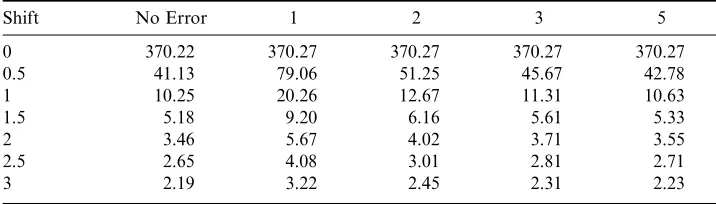
p2_m/p2ó1. We observe that as the value of B increases, the eff_{ect on the ARL}

diminishes. This result is again in accordance with Linna & Woodall (2001). Furthermore, in both Tables 1 and 2 the eff_{ect of the measurement error on the}

ARL values lessens as the shift increases. We have to state also thatA does not aff_{ect the ARL performance in this study.}

Table 2.ARL for the covariate model for diff_{erent values ofB}

Shift No Error 1 2 3 5

0 370.22 370.27 370.27 370.27 370.27 0.5 41.13 79.06 51.25 45.67 42.78

1 10.25 20.26 12.67 11.31 10.63

1.5 5.18 9.20 6.16 5.61 5.33

2 3.46 5.67 4.02 3.71 3.55

2.5 2.65 4.08 3.01 2.81 2.71

Table 3.ARL for multiple measurementskó5,Bó1 for diff_{erent values ofp2}

m/p2

Shift No Error 0.1 0.2 0.3 0.5 1 0 370.22 370.26 370.26 370.27 370.27 370.27 0.5 41.13 41.96 42.78 43.59 45.22 49.26 1 10.25 10.44 10.63 10.82 11.21 12.18 1.5 5.18 5.25 5.33 5.41 5.57 5.96

2 3.46 3.51 3.55 3.60 3.69 3.91

2.5 2.65 2.68 2.71 2.74 2.80 2.94

3 2.19 2.21 2.23 2.25 2.29 2.40

In Table 3, we can see the ARL results for the covariate model with multiple measurements for diff_{erent values of p2}

m/p2when kó5 and Bó1. It is obvious

that if the practitioner has the ability to take five measurements in each unit then for values of p₂

m/p2 less than 0.3 we may say that the process operates

actually without measurement error. For values larger than 0.3 the eff_{ect is}

seriously reduced in comparison to the kó1 case, which corresponds to the results in Table 1, even forp₂

m/p2ó1. Table 4 presents the results in the case of

multiple measurements for diff_{erent values of B. We see that, as the value of B}

increases, the eff_{ect on the ARL diminishes. This result is in accordance with the}

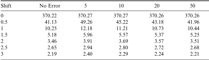
results in Table 2. Moreover, in Table 5 we have results in the case of multiple measurements for diff_{erentkvalues. As the value ofkincreases, the measurement}

error eff_{ect reduces. However, since the cost and time needed for the extra}

Table 4.ARL for multiple measurementskó5,p₂

m/p2ó1 for different values ofB

Shift No Error 1 2 3 5

0 370.22 370.27 370.26 370.28 370.27 0.5 41.13 49.26 43.18 42.05 41.46

1 10.25 12.18 10.73 10.46 10.33

1.5 5.18 5.96 5.37 5.26 5.21

2 3.46 3.91 3.57 3.51 3.48

2.5 2.65 2.94 2.72 2.68 2.66

3 2.19 2.40 2.24 2.21 2.20

Table 5.ARL for multiple measurements for diff_{erent values ofk}

Shift No Error 5 10 20 50

0 370.22 370.27 370.27 370.26 370.26 0.5 41.13 49.26 45.22 43.18 41.96

1 10.25 12.18 11.21 10.73 10.44

1.5 5.18 5.96 5.57 5.37 5.25

2 3.46 3.91 3.69 3.57 3.51

2.5 2.65 2.94 2.80 2.72 2.68

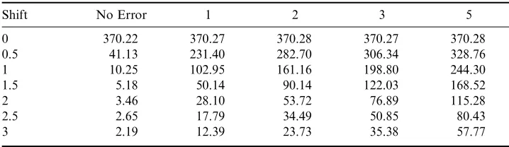
Table 6.ARL for linearly increasing variance for diff_{erent values ofD}

Shift No Error 1 2 3 5

0 370.22 370.27 370.28 370.27 370.28 0.5 41.13 231.40 282.70 306.34 328.76 1 10.25 102.95 161.16 198.80 244.30 1.5 5.18 50.14 90.14 122.03 168.52

2 3.46 28.10 53.72 76.89 115.28

2.5 2.65 17.79 34.49 50.85 80.43

3 2.19 12.39 23.73 35.38 57.77

measurements are important factors, the practitioner will have to do a trade-off

between these two concerns and the measurement error s/he can put up with. We have to stress here that the results displayed in this case are for the worst case, since we chooseBó1 andp₂

m/p2ó1, which correspond to the most affected

combination. Therefore, one may conclude that the results in the other cases will be even better.

The results in the case of linearly increasing variance are displayed on Tables 6 and 7. In Table 6 we have the ARL values whenBó1,Có0 andp₂

m/p2ó1 for

diff_{erent values of D. We see that even for small values of D there is a more}

serious eff_{ect than in the no error case. Additionally, as the value ofDincreases,}

this eff_{ect is getting larger. This result is expected because, as D increases, so}

does the variance of the error component in the model. In this special case of measurement error, extra precaution is needed because the ability of the EWMA chart to detect fast small shifts is cancelled out. Consequently, serious distortion factors may go undetected for a long time, costing a lot in money, time and credibility. Table 7 presents the ARL results whenBó1,Dó1 andp2_m/p2ó1 for diff_{erent values of C. Analogously to Table 6, increasing values of C cause an}

increasing measurement error eff_{ect on the ARL. However, this e}ff_{ect is not of}

the same magnitude as the eff_{ect of D. This result is also expected since D is}

multiplied by the mean, increasing faster than the error variance asDincreases whereasC is just added to this variance.

In all the computations we used 211 states for the Markov Chain method. Moreover, the values of the constants are ó0.25 and Ló2.898. In order to

Table 7.ARL for linearly increasing variance for diff_{erent values ofC}

Shift No Error 0 1 2 3

0 370.22 370.27 370.29 370.27 370.27 0.5 41.13 231.40 239.08 245.96 252.14 1 10.25 102.95 110.13 116.95 123.44 1.5 5.18 50.14 54.53 58.84 63.06

2 3.46 28.10 30.72 33.34 35.95

2.5 2.65 17.79 19.43 21.09 22.75

detect small shifts fast thevalue usually used is 0.1 or less. However such small values are not able to detect small to moderate shifts and this is the reason for thevalue chosen. Note also that in all the cases the control limits used are the ones with the limiting values.

Conclusions

In this paper, the performance of the EWMA control chart for the mean, when there is a measurement error eff_{ect, assuming a model with covariates, was}

presented. It was found that this error can aff_{ect the ARL performance of this}

chart. Multiple measurements proved to be a solution to this problem. However, the extra money and time needed is another problem. A properly designed economic study on this matter in each specific problem may reveal the possibility of such an action. On the other hand, the additional time needed may not be a problem since, in today’s industry, the measurements are usually done in an automated way. Linearly increasing variance was also discussed and proved to be the type of measurement error that aff_{ects the performance of the chart to a}

larger extent.

References

Borror, C. M., Montgomery, D. C. & Runger, G. C. (1999) Robustness of the EWMA control chart to non-normality,Journal of Quality Technology, 31, pp. 309–316.

Crowder, S. V. (1987) A simple method for studying run length distributions of exponentially weighted moving average control charts,Technometrics, 29, 401–407.

Champ, C. W. & Rigdon, S. E. (1991) A comparison of the Markov Chain and the integral equation approaches for evaluating the run length distribution of quality control charts,Communications in Statistics-Simulation and Computation, 20, pp. 191–204.

Domangue, R. & Patch, S. C. (1991) Some omnibus exponentially weighted moving average statistical process monitoring schemes,Technometrics, 33, pp. 299–313.

Gan, F. F. (1998) Designs of one and two sided exponential EWMA charts,Journal of Quality Technology, 30, pp. 55–69.

Henderson, R. G. (2001) EWMA and industrial applications to feedback adjustment and control,Journal of Applied Statistics, 28, pp. 399–407.

Linna, K. W. & Woodall, W. H. (2001) Effect of measurement error on Shewhart control charts,Journal of Quality Technology, 33, pp. 213–222.

Linna, K. W., Woodall, W. H. & Busby, K. L. (2001) The performance of multivariate control charts in the presence of measurement error,Journal of Quality Technology, 33, pp. 349–355.

Lucas, J. M. & Saccucci, M. S. (1990) Exponentially weighted moving average control schemes: properties and enhancements,Technometrics, 32, 1–12.

Mittag, H.-J. & Stemann, D. (1998) Gauge imprecision effect on the performance of the -S control chart, Journal of Applied Statistics, 25, pp. 307–317.

Montgomery, D. C. & Runger, G. C. (1994) Gauge capability and designed experiments. Part I: basic methods,Quality Engineering, 6, pp. 115–135.

Ng, C. H. & Case, K. E. (1989) Development and evaluation of control charts using exponentially weighted moving averages,Journal of Quality Technology, 21, pp. 242–250.

Reynolds, M. R. Jr. (1996) Shewhart and EWMA variable sampling interval control charts with sampling at fixed times,Journal of Quality Technology, 28, pp. 199–212.

Steiner, S. H. (1999) EWMA control charts with time-varying control limits and fast initial response, Journal of Quality Technology, 31, pp. 75–86.

Stoumbos, Z. G. & Sullivan, J. H. (2002) Robustness to non-normality of the multivariate EWMA control chart,Journal of Quality Technology, 34, pp. 260–276.

Appendix

In order to compute the probability density function, the cumulative distribution function and the first moment of the run length distribution of the EWMA chart for the mean we may approximate it as a discrete Markov Chain by dividing the distance between the control limits in 2mò1 states, each of which has width 2. We say that the statisticZ

tremains in statejas long asSjñ\Zt\Sjòwhere

ñmOjOmandS

jis the midpoint in thejth interval. WhenZtcrosses the control

limits we say that it is in the absorbing state. On the other hand, when the process is in control we say that it is in a transient state.

The transition probability matrixfor the EWMA chart for the mean is computed as

Pó

0_T 1

whereRis a sub-matrixcontaining the transient states,Iis atîtidentity matrix and1is a tî1 vector of unities. The jkth element of the sub-matrixR is given byp

jkóP¨Sjñd\jyiò(1ñj)SjOSjòd≠. In the case of the normal distribution

with the assumed model with covariates of our case the probabilities are given by

p jkó'

(S

kjòd)ñ(1ñj)SKñj(AòBk)

j(B2p₂òp₂

m)/n

ó'

m)/n

.

When we have multiple measurements the probabilities are

p jkó'

(S

kjòd)ñ(1ñj)SKñj(AòBk)

j(B2p/n2òp₂

m/nk

ó'

m/nk

and in the case of linearly increasing variance the probabilities are

p jkó'

(S

kjòd)ñ(1ñj)SKñj(AòBk)

j(B2p₂òCòDk)/n

(S

kjñd)ñ(1ñj)SKñj(AòBk)

j(B2p₂òCòDk)/n

Letdenote the run length of the EWMA thenP(Ot)ó(IñRt)1and therefore

P(ót)ó(Rt1ñRt)1 for tP1. The ARL can be computed using the formula

E(q)ó&