Asymptotic Solving Essentially Nonlinear Problems

(1)

Asymptotic Solving Essentially Nonlinear Problems

Alexander D. Bruno

Department of Singular Problem, Keldysh Institute of Applied Mathematics of RAS, Miusskaya sq. 4, 125047, Moscow, Russia

Abstract

Here we present a way of computation of asymptotic expansions of solutions to algebraic and dif-ferential equations and present a survey of some of its applications. The way is based on ideas and algorithms of Power Geometry. Power Geometry has applications in Alge-braic Geometry, Differential Algebra, Nonstandard Analysis, Microlocal Analysis, Group Analysis, Tropical/Idempotent Mathematics and so on. We also discuss a connection of Power Geometry with Idempotent Mathematics.

Keywords

Singularity, Newton Polyhedron, Painlev´e Equation, Boundary Layer, Idempotent Analysis

1 Introduction

We develop a new Calculus based on Power Geometry [1–4]. At present, it allows to compute local and asymp-totic expansions of solutions to nonlinear equations of three classes:

1. algebraic,

2. ordinary differential, 3. partial differential,

as well as to systems of such equations. However, it can also be extended to other classes of nonlinear equations: func-tional, integral, integro-differential etc.

Principal ideas and algorithms are common for all classes of equations. Computation of asymptotic expansions of solu-tions consists of 3 following steps (we describe them for one equationf = 0).

1. Calculation of truncated equationsfˆ_j(d)= 0by means of generalized faces of the convex polyhedronΓ(f)which is a generalization of the Newton polyhedron. The first term of the expansion of a solution to the initial equa-tionf = 0is a solution to the corresponding truncated equationfˆ_j(d)= 0.

2. Finding solutions to a truncated equation fˆ_j(d) = 0, which is quasihomogenous. Using power and logarith-mic transformations of coordinates we can reduce the equation fˆ_j(d) = 0 to such simple form that can be

solved. Among the solutions found we should select ap-propriate ones which yield the first terms of asymptotic expansions.

3. Computation of the tail of the asymptotic expansion. Each term in the expansion is a solution of a linear equa-tion which can be written down and solved.

Indeed Power Geometry (as a basis of Nonlinear Analysis) can be considered as the third level of Differential Calculus (after Classical Analysis and Functional Analysis). Elements of Plane Power Geometry were proposed by Newton for alge-braic equation (1670) [5]; and by Briot and Bouquet for ordi-nary differential equation of the first order (1856) [6]. Space Power Geometry for a nonlinear autonomous system of Ordi-nary differential equations (ODEs) was proposed by the au-thor (1962) [1], and for a linear partial differential equation (PDE), by Mikhailov (1963) [7]. Thus, in 2012 we could cel-ebrate 50 years of the first publication on theNewton polyhe-dron.

Back in the autumn of 1959, I was a third-year stu-dent of Department of Mechanics and Mathematics of the Lomonosov Moscow State University, and invented a poly-hedron to study asymptotic behavior of solutions to an au-tonomous system of ODEs near a degenerated stationary point. The polyhedron was described in my work, which was presented at a students’ works competition in 1961. In that year Arnold was a postgraduate student, and he became a referee of my work. He estimated my works as not very good, for the mere reason that “geometry of power exponents is useless”. In 1962-1970, Arnold wrote reports on some of my articles with the same (rather negative) evaluation of Power Geometry. See details in Section 6 of Chapter 8 of English Edition of my book [3]. However, in 1973 Arnold re-introduced my polyhedron as “Newton polyhedron” and that looked as if he was the inventor of the polyhedron. In fact, he invented only the name [8]. V.P. Maslov was very surprised when I told him (in 1990) that the Newton polyhe-dron was my invention (he thought that it was Arnold’s).

(2)

l

k

1 0

[image:2.595.107.217.64.179.2]

1

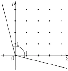
Figure 1.Set of power exponentsk, lin expansion of Type 2

2 Algebraic Equations [2, 3]

We consider a polynomial depending on three variables near its singular point where the polynomial vanishes with all the first partial derivatives. We propose a method of com-putation of asymptotic expansions of all branches of the set of roots of the polynomial near the above mentioned singular point. There are three types of expansions. The method of computation is based on the spatial Power Geometry. Most of our examples are for polynomials in two variables.

2.1

The Problem Statement

LetX = (x, y, z)∈R3orC3andg(X)be a polynomial.

Definition 1 A pointX0 is called singular for the setG =

{X :g(X) = 0}if all the partial derivatives of the first order of the polynomialgvanish in the pointX0andg(X0) = 0.

Problem 1 Near the singular pointX0= 0for each branch

of the setG, find a parameter expansion of one of the follow-ing three types.

Type 1

x=

∞

∑

k=1

bkvk, y= ∞

∑

k=1

ckvk, z= ∞

∑

k=1

dkvk,

wherebk, ck, dkare constants.

Type 2

x=∑bklukvl, y=∑cklukvl, z=∑dklukvl,

wherebkl, ckl, dklare constants and integer points(k, l)

are in a sector with the angle less thanπ(see Fig. 1).

Type 3

x=

∞

∑

k=0

βk(u)vk, y= ∞

∑

k=0

γk(u)vk, z= ∞

∑

k=0

δk(u)vk,

whereβk(u),γk(u),δk(u)are rational functions ofu

and√ψ(u), andψ(u)is a polynomial inu.

2.2

Objects and algorithms of Power Geometry

Consider a finite sum (for example, a polynomial) g(X) =∑gQXQoverQ∈S(g), (1)

where X = (x, y, z) ∈ C3_, _Q _{= (}_q

1, q2, q3) ∈ R3 and

XQ ₌ _xq1_yq2_zq3_,_g

Q = const ∈ C\{0}. To each of the terms of sum (1), we assign itsvector power exponentQ, and to the whole sum (1), we assign the set of all vector power ex-ponents of its terms, which is called thesupportof sum (1) or of the polynomialg(X), and it is denoted byS(g). The con-vex hull of the supportS(g)is called theNewton polyhedron

of the sumg(X), and it is denoted byΓ(g). The boundary∂Γ

of the polyhedronΓ(g)consists ofgeneralized faces1Γ(_jd)of various dimensionsd = 0,1,2. Herej is the number of a face. To each generalized faceΓ(_jd), we assign thetruncated sumgˆ_j(d)(X) =∑gQXQ_over_Q_∈_Γ(d)

j ∩S(g).

Example 1: support and the Newton polygon

We consider the polynomial g(x, y) = x3₊_y3₋₃_xy.

SupportS(g)consists of points Q1 = (3,0),Q2 = (0,3),

Q3 = (1,1). The Newton polygon Γ(g) is the triangle

Q1Q2Q3 (Fig. 2). Its edges and corresponding truncated

polynomials are

Γ(1)₁ : ˆg₁(1)=x3−3xy, Γ(1)₂ : ˆg(1)₂ =y3−3xy,

Γ(1)₃ : ˆg(1)₃ =x3+y3.

Let R3

∗ be a space dual to the space R3 and P =

(p1, p2, p3)be points of this dual space. Thescalar product

⟨Q, P⟩=q1p1+q2p2+q3p3 (2)

is defined for the pointsQ∈R3_and_P _∈_R3

∗. In particular, the external normalNkto the generalized faceΓ(_kd)is a point (vector) inR3

∗.

The scalar product⟨Q, Nk⟩reaches the maximum value at the pointsQ ∈ Γ(_kd)∩S(g), i. e. at the points of the gen-eralized faceΓ(_kd). The set of all pointsP ∈ R3

∗, at which the scalar product (2) reaches the maximum overQ ∈S(g)

exactly at pointsQ∈Γ(_kd), is callednormal coneof the gen-eralized faceΓ(_kd)and is denoted byU(_kd).

Example 2: Normal Cones (cont. of Example 1)

For facesΓ(_jd)of the Newton polygonΓ(g)of Fig. 2, nor-mal cones are shown in Fig. 3.

Γ(1)₂

Γ(1)₁

1 2 3 q2

1 2 3

q1

0

Q1 Q2

Q3

[image:2.595.363.474.599.710.2]

Γ(1)₃

Figure 2.The Newton polygon of polynomialx3₊_y3_{= 3}_xy_.

For edge Γ(1)_j , j = 1,2,3, normal coneU(1)_j is the ex-ternal ray orthogonal to this edge. For vertex Γ(0)_j = Qj, j= 1,2,3, normal cone is open sector between external rays orthogonal to edgesΓ(1)_k adjacent to vertexQj.

(3)

p2

p1 U(0)₂

U(0)₁ U(0)₃

U(1)₁ U(1)₂

[image:3.595.123.234.64.175.2]

U(1)₃

Figure 3.Normal conesU(_jd)for polygon of Fig. 2

Theorem 1 ( [3]) If fort→ ∞the curve

x=btp1_{(1 +}_o₍₁₎₎_{, y}₌_ctp2_{(1 +}_o₍₁₎₎_{, z}₌_dtp3_{(1 +}_o₍₁₎₎_,

(3)

where b, c, dand pi are constants, belongs to the set G =

{X:g(X) = 0}, and the vectorP = (p1, p2, p3)belongs to

U(_kd), then the first approximationx= btp1_,_y ₌_ctp2_,_z ₌

dtp3 _{of curve}₍₃₎_{satisfies the truncated equation}_ˆ_g(d)

k (X) =

0.

The truncated sumˆg(0)_j corresponding to the vertexΓ(0)_j is a monomial. Such truncations are of no interest and will not be considered. We will consider truncated sums correspond-ing to edgesΓ(1)_j and facesΓ(2)_j only.

Power transformationsare mappings of the form

logX=B logX1, (4)

where logX = (logx,logy,logz)T, logX1 =

(logx1,logy1,logz1) T

, B is a non-degenerate square

3×3matrix(bij)with rational elementsbij (they are often integer).

The monomialXQ _{is transformed to the monomial}_XQ1

1

by power transformation (4), whereQT

1 = BTQT. Power

transformations and multiplications of polynomial by mono-mial generate the affine geometry in space R3 _{of vector}

power exponents of polynomial monomials. The matrix B with integer elements anddetB=±1is calledunimodular.

Theorem 2 ( [3]) For the face Γ(_jd), there exists a power transformation(4)with an unimodular matrixBwhich trans-forms the truncated sumgˆ_j(d)(X)into the sum ind coordi-nates, i. e. ˆg(_jd)(X) = X₁Qh(X1), whereh(X1) = h(x1)

if d = 1, and h(X1) = h(x1, y1)if d = 2. Here Q =

(q1, q2, q3)∈R3and other coordinatesy1,z1ford= 1and

z1ford= 2are small. Ifˆg (d)

j (X)is a polynomial, then the

sumh(X1)is a polynomial as well.

2.3

Cone of the problem

Thecone of the problemLis a convex cone of such vectors P = (p1, p2, p3)∈R3_∗

that curves of form (3) fill those part of the space (x, y, z)

which is under consideration, i. e. must be studied.

So, our initialProblem 1corresponds to the cone of the problem

L={P = (p1, p2, p3) :P <0}

inR3_∗, sincex, y, z→0(andx, y, zas in (3)).

Ifx→ ∞thenp1>0in the cone of the problemL.

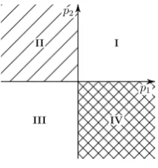
Example 3: Cont. of Examples 1 and 2

For variables x, y near origin x = y = 0 cone of the problem is the quadrant III: L3 = {p1, p2 < 0}, near

in-finityx = y = ∞ cone of the problem is the quadrant I:

L1 = {p1, p2 > 0}, near pointx= 0,y =∞cone of the

problem is the quadrant II:L2 ={p1 <0, p2>0}(Fig. 4).

In Fig. 3 some cones of the problem Li intersects several normal conesU(2)_j . E.g. L3intersectsU

(1) 1 ,U

(1) 2 andU

(0) 1 ,

U(0)₂ ,U(0)₃ .L1intersectsU (1) 3 ,U

(0) 1 ,U

(0)

2 .

p₂

p₁

IV III

II I

Figure 4.Cones of the problem.

2.4

Steps for Problem solving

Step 1. We compute the supportS(g), the Newton polyhe-dronΓ(g), its two-dimensional facesΓ(2)_j and their ex-ternal normalsNj. Using normalsNj we compute the normal conesU(1)_k to edgesΓ(1)_k .

Step 2. We find all the edgesΓ(1)_k and facesΓ(2)_j , whose nor-mal cones intersect the cone of the problem L. It is enough to select all the facesΓ(2)_j , whose external nor-malsNj intersect the cone of the problemL, and then add all the edgesΓ(1)_k of these faces.

Step 3.

• For each of the selected edgesΓ(1)_k , we perform a power transformationX →X1of Theorem 2 and

we get the truncated equation in a formh(x1) = 0.

• We find the roots of this equation. Letx0₁ be one of its roots.

• We perform the power transformationX →X1in

the whole polynomialg(X)and we get the poly-nomialg1(X1) =g(X).

• We make the shift of variablesx2=x1−x01,y2=

y1,z2 =z1 in the polynomialg1(X)and get the

polynomialg2(X2) =g1(X1).

• Ifx0

1is a simple root of the equation h(x1) = 0

then, according to the Implicit Function Theorem, it corresponds to an expansion of the formx2 =

∑

aklyk1zl1, where akl are constants. It gives an expansion of type 2 in coordinatesX.

• Ifx0₁is a multiple root of the equationh(x1) = 0

then we compute the Newton polyhedron of the polynomialg2(X2), compute the new cone of the

problemL2as the convex cone generated by

[image:3.595.376.489.194.314.2]

(4)

Step 4.

• For each of the selected facesΓ(2)_j , we perform a power transformationX → X1 of Theorem 2

and we get a truncated equation in the form h(x1, y1) = 0.

• We factorize h(x1, y1) into prime factors. Let

˜

h(x1, y1)be one of such factors and its algebraic

curve has genusρ.

• Ifρ = 0then there exists birational uniformiza-tionx1 = ξ(y2),y1 = η(y2) of this curve. We

change variablesx1 = ξ(y2) +x2, y1 = η(y2)

and thenh˜is divided byx2. We change variables

in the whole polynomialg(X)and get the polyno-mialg2(X2)

def

= g1(X1) =g(X).

• If˜h(x1, y1)is simple factor ofh(x1, y1)then roots

of the polynomialg2(X2)are expanded into series

of the form

x2=

∞

∑

k=1

αk(y2)z2k, (5)

whereαk(y2)are rational functions ofy2. It gives

an expansion of type 3 in original coordinatesX.

• If˜h(x1, y1)is a multiple factor ofh(x1, y1)then

we compute the Newton polyhedron of the poly-nomialg2(X2), compute the cone of the problem

L2 = {P : p2, p3 < 0} and continue

computa-tions.

• Ifρ= 1(elliptic curve), there exists the birational change of variablesx1, y1 →x2, y2transforming

˜

h(x1, y1)into the normal formx22−ψ(y2), where

ψis a polynomial of order 3 or 4.

• Ifρ > 1, we distinguish hyper-elliptic and non hyper-elliptic curves. The hyper-elliptic curve is birationally equivalentx1, y1 →x2, y2to its

nor-mal formx22−ψ(y2), whereψis a polynomial of

order2ρ+ 1or2ρ+ 2.

• Ifρ>1and we have the (hyper)elliptic curve and factorh˜ofhis simple we get expansions of solu-tions of equationg2(X2) = 0into series (5), where

αk are rational functions ofy2and

√

ψ(y2). We

get the expansion of type 3 in original coordinates X.

• Ifρ>1and we have the (hyper)elliptic curve and

˜

h(x1, y1)is a multiple factor ofh(x1, y1)then we

continue forg2(X2)as above.

In this procedure we distinguish two cases:

Case 1. Truncated polynomial contains linear part of one of the variables orx0

1is a simple root ofh(x1)or˜h(x1, y1)

is simple factor ofh(x1, y1). Then a generalization of

Implicit Function Theorem is applicable and it is possi-ble to compute parametric expansion of set of roots of full polynomial.

Case 2. Truncated polynomial does not contain linear part of any variable and x01 is a multiple root of h(x1) or

˜

h(x1, y1) is a multiple factor of h(x1, y1). Then the

Newton polyhedron for full polynomial must be built and we must consider new truncated polynomials tak-ing into account the new cone of the problemL.

Example 4 (cont. of Examples 1–3)

• For edgeΓ(1)₁ , we get truncated equationx2₋₃_y _{= 0}_,

i. e. y = x2/3. It is the case 1, and this asymptotic form is continued into power expansion of branchy =

x2/3 +∑∞_k₌₂bkx2knear the originx=y= 0.

• For edgeΓ(1)₂ , we get truncated equationy2₋₃_x_{= 0}_,

i. e. y =±√3x. It is the case 1, and these asymptotic forms are continued into power expansions of branches y=±√3x+∑∞_k₌₂bkxk/2_{near the origin}_x₌_y_{= 0}_.

• For edgeΓ(1)₃ , we get truncated equationx3₊_y3 _{= 0}_.

It has the simple factorx+y = 0, i. e. y =−x. It is again case 1 of simple root, and the power expansion at infinityy=−x−1 +∑∞_k₌₁bkx−k_{gives the asymptote} x+y =−1for the curveg(x, y) = 0calledfolium of

Descartes(Fig. 5).

−1

1 2 y

−1 1 2

[image:4.595.361.472.369.485.2]

x

Figure 5.Folium of Descartes

Asymptotic description of a subset of singular points ofG can be obtained by the same procedure, but we have to select only singular points in each truncated equation. As result we obtain expansions of type 1.

2.5

Results

Theorem 3 ( [4]) The algorithm of Subsection 2.4, in the case when all curves formed by roots of corresponding two-dimensional truncated equations with positive genus are el-liptic or hyper-elel-liptic, yields a local description of all com-ponents of the set G, adjacent to the starting pointX0, in

form of expansions of types 1–3.

2.6

Implementation and Application

(5)

Example 5 [9]

g(X) = 512z6−4352z5y−768z5x+ 14848z4y2

+ 5376z4yx+ 512z4x2−25408z3y3−14656z3y2x

−2752z3yx2−192z3x3+ 21800z2y4

+ 19168z2y3x+ 5360z2y2x2+ 736z2yx3+ 40z2x4

−7500zy5−11700zy4x−4376zy3x2−904zy2x3

−92zyx4−4zx5+ 2500y5x+ 1200y4x2

+ 344y3x3+ 48y2x4+ 4yx5−256z5+ 2880z4y

+ 1344z4x−14976z3y2−6720z3yx−1344z3x2

+ 37928z2y3+ 13816z2y2x+ 5144z2yx2

+ 456z2x3−45120zy4−14464zy3x−6784zy2x2

−1152zyx3−64zx4+ 20250y5+ 6490y4x

+ 3156y3x2+ 740y2x3+ 82yx4+ 2x5+ 1872z4

+ 2016z3y−5088z3x−35496z2y2+ 15888z2yx

+ 2200z2x2+ 67608zy3−12936zy2x−5176zyx2

−344zx3−37827y4+ 828y3x+ 2782y2x2

+ 412yx3+ 13x4−13824z3+ 62208z2y

+ 6912z2x−93312zy2−20736zyx−1152zx2

+ 46656y3+ 15552y2x+ 1728yx2+ 64x3.

[image:5.595.90.264.418.558.2]

The structure of solutions of the algebraic equation g(X) = 0near its singular points (including infinity). The Newton polyhedron of this equation is shown on Fig. 6.

Figure 6.The Newton polyhedron for polynomialg(X).

Near originX = 0we obtain

x=

∞

∑

k=0

βk(u)vk, y= ∞

∑

k=0

γk(u)vk, z= ∞

∑

k=0

δk(u)vk,

whereβk(u),γk(u),δk(u)are rational functions ofu. More precisely, we have:

x= Ω1(u)

(

12v3+ 18Ω2(u)

27u2_{+ 10}_u₋₅

u+ 1 v

4

)

+o(v4),

y= Ω1(u)

(

2v2+ 12Ω2(u)(5u−1)v3

)

+o(v3),

z= Ω1(u)

(

3v2+ 4Ω2(u)

71u2+ 13u−4 3u+ 1 v

3

)

+o(v3)

here Ω1(u) =

54(3u+ 1)3

(7u+ 1)(u+ 1)2, Ω2(u) =

3u+ 1

(7u+ 1)(u+ 1).

3 Ordinary

Differential

Equations.

Algebraic Approach

3.1

Plane Power Geometry [11]

First, consider one differential equation and power expan-sions of its solutions (later we consider more complicated ex-pansions).

Letxbe independent andybe dependent variables,x, y∈

C. Adifferential monomiala(x, y)is a product of an ordinary monomialcxq1_yq2_{, where}_c_{= const}∈C_,₍_q

1, q2)∈R2, and

a finite number of derivatives of the formdl_y/dxl_,_l _∈_N_{. A} sum of differential monomials

f(x, y) =∑ai(x, y) (6) is called thedifferential sum.

Problem 2 Let a differential equation be given

f(x, y) = 0, (7)

wheref(x, y)is a differential sum. Asx→0, or asx→ ∞, for solutionsy=φ(x)to equation(7), find all expansions of the form

y=crxr+

∑

csxs, cr= const∈C, cr̸= 0, (8)

where cs are polynomials in logx, and power exponents r, s∈R,ωr > ωs, andω=−1, ifx→0, orω= 1, ifx→

∞.

The procedure to compute expansions (8) consists of two steps: computation of the first approximations y = crxr_, cr̸= 0and computation of further expansion terms in (8).

To each differential monomiala(x, y), we assign its (vec-tor)power exponentQ(a) = (q1, q2)∈R2by the following

rules:

Q(cxq1_yq2_{) = (}_q

1, q2); Q(dly/dxl) = (−l,1);

when differential monomials are multiplied, their power ex-ponents must be added as vectorsQ(a1a2) =Q(a1)+Q(a2).

The set S(f) of power exponents Q(ai) of all differential monomialsai(x, y)presented in differential sum (6) is called thesupport of the sumf(x, y).

Obviously,S(f)∈R2. The convex hullΓ(f)of the sup-port S(f) is called the polygon of the sum f(x, y). The boundary∂Γ(f)of the polygonΓ(f)consists of the vertices

Γ(0)_j and the edgesΓ(1)_j . They are called (generalized)faces

Γ(_jd), where the upper index indicates the dimension of the face, and the lower one is its number. Each faceΓ(_jd) corre-sponds to thetruncated sum

ˆ

f_j(d)(x, y) =∑ai(x, y)overi:Q(ai)∈Γ(_jd)∩S(f) (9) and totruncated equationfˆ_j(d)(x, y) = 0of equation (7).

Example 6

Consider the third Painlev´e equation

(6)

q2

−1 0 1

q1 Q1

Q2

Q3

Q4

Q5

Γ(1)₁ Γ(1)₂

[image:6.595.106.219.65.176.2]

Γ(1)₃

Figure 7.The Newton polygon of equation (10)

assuming the complex parametersa,b,c,d ̸= 0. Here the first three differential monomials have the same power ex-ponent Q1 = (−1,2), then Q2 = (0,3), Q3 = (0,1),

Q4 = (1,4), Q5 = (1,0). They are shown in Fig. 7 in

coordinatesq1,q2.

Their convex hullΓ(f)is the triangle with three vertices

Γ(0)₁ = Q1,Γ (0)

2 = Q4, Γ (0)

3 = Q5, and with three edges

Γ(1)₁ ,Γ(1)₂ ,Γ(1)₃ . The vertex Γ(0)₁ = Q1corresponds to the

truncation

ˆ

f₁(0)(x, y) =−xyy′′+xy′2−yy′,

and the edgeΓ(1)₁ corresponds to the truncation

ˆ

f₁(1)(x, y) = ˆf₁(0)(x, y) +by+dx. (11) Let the planeR2_∗be dual to the planeR2such that forP = (p1, p2)∈R2_∗andQ= (q1, q2)∈R2, the scalar product

⟨P, Q⟩def= p1q1+p2q2

is defined. Each face Γ(_jd) corresponds to its own normal coneU(_jd) ⊂ R2_∗ formed by the external normal vectorsP to the faceΓ(_jd). For the edgeΓ(1)_j , the normal coneU(1)_j is the ray orthogonal to the edgeΓ(1)_j and directed outward the polygonΓ(f). For the vertexΓ(0)_j , the normal coneU(0)_j is the open sector (angle) in the planeR2_∗with the vertex at the originP = 0and limited by the rays which are the normal cones of the edges adjacent to the vertexΓ(0)_j .

Example 7 (cont. of Example 6)

For equation (10), the normal conesU(_jd)of the facesΓ(_jd)

are shown in Fig. 8.

p2

p1 U(0)₂

U(0)₃ U(0)₁

U(1)₁ U(1)₂

U(1)₃

Figure 8.The normal conesU(_jd)for polygon of Fig. 7

Thus, each faceΓ(_jd)corresponds to the normal coneU(_jd)

in the planeR2_∗and to the truncated equationfˆ_j(d)(x, y) = 0.

Theorem 4 ( [11]) If expansion (8) satisfies equation (7), and ω(1, r) ∈ U_j(d), then the truncation y = crxr of

so-lution(8)is the solution to truncated equation(9).

As truncated equation is quasi–homogeneous it is not dif-ficult to find its power solutions. Hence, to find all truncated solutions y = crxr to equation (7), we need to compute: the support S(f), the polygonΓ(f), all its facesΓ(_jd), and their normal conesU(_jd). Then for each truncated equation

ˆ

f_j(d)(x, y) = 0, we need to find all its solutionsy = crxr which have one of the vectors ±(1, r)lying in the normal coneU(_jd).

For each power solutiony =crxrof the truncated equa-tionfˆ_j(d)= 0, we can compute itscharacteristic polynomial

ν(k). Rootskjofν(k)withωkj < ωrarecritical numbers

of the solutioncrxr_.

Example 8 (cont. of Examples 6, 7)

For the truncated equationfˆ₁(0) = 0withω=−1, we have solutionsy=crxr_{with arbitrary constants}_r_and_{cr. But} ac-cording to Theorem 4,y=crxr_{can be a formal asymptotic} form of a solution to full equation (7) if ω(1, r) ⊂ U(0)₁ , i. e. −1 < r <1. Corresponding characteristic polynomial ν(k) =−(k−r)2_{. Hence, here we have no critical numbers.}

For the truncated equationfˆ₁(1) = 0, we have power so-lutiony = −dx/b. Its characteristic polynomial isν(k) =

(k−1)2₊_b2_/d. _.

Using supportS(f)of the equation (7) and critical num-bers k1, . . . , k_κ with ωr > ωki, we can find the set

K(k1, . . . , kκ)⊂ R,support of expansion(8). Its elements

ssatisfy the inequalityωr > ωs.

Theorem 5 ( [11]) Ify =crxr_,_c_{= const}_,_ω₍₁_{, r}₎_∈_U(d) j ,

is a power solution to truncated equation (9), then equa-tion(7)has an expansion of solutions of the form

z=crxr+

∑

csxs over s∈K(k1, . . . , kκ), (12)

wherek1, . . . , kκ are critical numbers of the truncated

so-lution y = crxr; cs are polynomials in logx, which are

uniquely determined for s ̸= ki. If all critical numbers k1, . . . , kκare simple roots, and eachkidoes not lie in the set

K(k1, . . . , ki−1, ki+1, . . . , kκ), then all coefficients cs are

constant; fors ̸=ki, they are uniquely determined; and for

s=ki, they are arbitrary.

Example 9 (cont. of Examples 6–8)

For the truncated solutiony =cxr_to_fˆ(0)

1 = 0, arbitrary

c̸= 0,r∈(−1,1)

K={s=r+l(1−r)+m(1+r), l, m∈N∪{0}, l+m >0}. (13) Since there are no critical numbers, then allcsare constant and uniquely determined in expansion (12).

[image:6.595.108.218.638.756.2]

(7)

ℑ(b/√−d) = 0, then there is a unique real critical number k1= 1+|b/

√

−d|, and

K(k1) ={s= 1+2l+m(k1−1), l, m∈N∪{0}, l+m >0}.

(14) Hence, if the numberk1is not odd, then allcsare constant and uniquely determined in expansion (12) fors ̸=k1, and

ck1 is arbitrary. Finally, ifk1is odd, thenK(k1) =K, and

in expansion (12)csis a uniquely determined constant ifs < k1;ck1is a linear function oflogxwith an arbitrary constant

term;csis a uniquely determined polynomial inlogxifs >

k1.

The truncated equationfˆ_j(d)(x, y) = 0can have non-power solutionsy =φ(x)which are the asymptotic forms for so-lutions to the initial equationf(x, y) = 0. These non-power solutions y = φ(x)may be found using power and loga-rithmic transformations. Power transformation is linear in logarithms and defined by

logx=b11logu+b12logv,

logy=b21logu+b22logv,

B= (

b11 b12

b21 b22

)

, bij ∈R,detB̸= 0.

It induces linear dual transformations in spacesR2 _and_R2

∗.

Logarithmic transformationhas the forms ξ= loguorη= logv.

Example 10 (cont. of Examples 6–9)

For the truncated equation (11) corresponding to the edge

Γ(1)₁ with the normal vector−(1,1), we make power trans-formation

logx= logu,

logy= logu+ logv,

B= (

1 0 1 1 )

,

i. e.x=u,y=uv. Sincey′=xv′+v,y′′=xv′′+2v′, then, cancelingxand collecting similar terms, the equation (11), becomes

−x2vv′′+x2v′2−xvv′+bv+d= 0. (15)

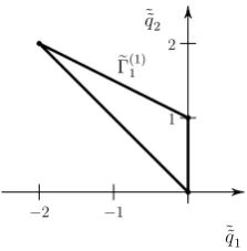
Its support consists of three pointsQe1= (0,2),Qe2= (0,1),

e

Q3= 0on the axisq˜1= 0(see Fig. 9).

˜

q₂

˜

q₁

0 1 2

Figure 9. The support and Newton polygon for the third Painlev´e equa-tion (15)

Now we make the logarithmic transformationξ = logx. Since v′ = ˙v/x, v′′ = (¨v −v˙)/x2, where ˙ = d/dξ,

1 2

˜˜

q₂

−2 −1

˜˜

q₁

[image:7.595.376.488.63.177.2]

e Γ(1)1

Figure 10.Support and Newton polygon of equation−vv¨+ ˙v2₊_bv₊_d_{= 0}_.

then, collecting similar terms, the equation (15) takes the form−vv¨+ ˙v2₊_bv₊_d_{= 0}_{. Its support and polygon are}

shown in Fig. 10. Applying the technique described before to this equation, we obtain the expansion of its solutionsv=

−(b/2)ξ2_{+ ˜}_cξ₊∑∞

k=0ckξ−k, where˜cis an arbitrary con-stant, and the constantsckare uniquely determined. In origi-nal variables, we obtain the family of non-power asymptotic formsy ∼x

[

−(b/2)(logx)2+ ˜clogx+ ∑∞

k=0

ck(logx)−k ]

of solutions to the initial equation (10), whenx→0.

3.2

Complex power exponents [11]

Indeed, the described method allows to calculate solutions with complex power exponents as well.

Thus, by the algebraic approach, expansions of solutions y=crxr+∑

s

csxs, (16)

with complex power exponentsrands, whereωℜr>ωℜs, and coefficientscrandcsare power series inlogx,log logx and so on, are found in a similar way.

In classical analysis, we encounter expansions in fractional powers and with constant coefficients, but here we obtain more complicated expansions of solutions.

3.3

Algorithms of Power Geometry

1. Computation of truncated equations and accompanying objects.

2. Solution of truncated equations. 3. Power transformations.

4. Logarithmic transformations.

5. Introducing independent variablexi_{instead of}_x. 6. Computation of the first variation of a sum.

7. Computation of expansions of solutions to the initial equation, beginning by solutions to a truncated equa-tion.

All these algorithms, except for 4 and 5, can be applied to solve algebraic equations.

(8)

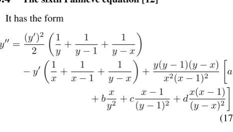
3.4

The sixth Painlev´e equation [12]

It has the form y′′= (y

′₎2

2 (

1

y +

1

y−1 + 1

y−x

)

−y′

( 1

x+

1

x−1 + 1

y−x

)

+y(y−1)(y−x)

x2₍_x−₁₎2

[

a

+bx y2 +c

x−1 (y−1)2 +d

x(x−1) (y−x)2

]

,

(17) wherea,b,c,dare complex parameters,xandy are com-plex variables,y′ =dy/dx. Equation (17) has three singular pointsx = 0, x = 1, andx = ∞. After multiplying by the common denominator, we obtain the equation as a differ-ential sum. Its support and its polygon, in the casea ̸= 0, b̸= 0, are shown in Fig. 11.

We found all formal asymptotic expansions (16) of solu-tions to equation (17) near its three singular points. They comprise 108 families. In particular, fora= 1/2andc= 0, there is an expansion of the form

y=− 1

cos[log(C1x)]

+ ∑

ℜs>1

csxs, (18)

where C1 is an arbitrary constant, the coefficients cs are

uniquely determined constants. Here

1/cos[log(x)] = 2/(xi+x−i) =

= 2xi ∞

∑

k=0

(

−x2i)k = 2x−i ∞

∑

k=0

(

−x−2i)k.

ForC1= 1and realx >0, solution (18) has infinitely many

poles accumulating at the pointx = 0. We also found all expansions of solutions to equation (17) near its nonsingular points. They comprise 17 families [13].

q

₂

q

₁

0

1

[image:8.595.47.281.68.201.2]

1

Figure 11.Support and Newton polygon for the sixth Painlev´e equation (17)

That approach was applied to ODE systems [14–17].

3.5

Applications

1. Asymptotic forms and expansions of solutions to the Painlev´e equations [12, 18, 19].

2. Periodic motions of a satellite around its mass center moving along an elliptic orbit [20].

3. New properties of motion of a top (rigid body with a fixed point) [21].

4. Families of periodic solutions of the restricted three-body problem and distribution of asteroids [22, 23]. 5. Integrability of ODE systems [24].

6. Surface waves on water [3, Ch. 5].

4 Ordinary

Differential

Equations.

Differential Approach

4.1

Orders of solutions and their derivatives

All solutions of the form (16) have the following property: pω

(

y(k)

)

=pω(y)−k, k= 1,2, . . . , n,

wherenis the maximal order of derivative in the initial ODE, and

pω(φ) =ωlim sup xω_→∞

log|φ(x)|

ωlog|x|

along fixedargx∈[0,2π)is theorder of the functionφ(x).

4.2

Differential Approach [25–30]

To each differential monomiala(x, y)we put in correspon-dence the 3D pointQ= (q1, q2, q3), whereq1andq2as

be-fore, butq3is the total order of derivatives in the monomial.

We obtain the 3D supporteS(f)of the initial ODEf = 0and polyhedron Γ(f)as convex hull ofS˜(f). Using truncated equations, corresponding to its faces and edges, we can find their solutions in the form of elliptic or hyperelliptic func-tionsφ0(x)and continue them into power-(hyper)elliptic

ex-pansion

y=φ0(x) +

∞

∑

l=1

φl(x)x−ωl, (19) where all φl(x)are elliptic or hyperelliptic functions. This differential approach allows to find expansions (19) for so-lutions with property pω

(

y(k)) ₌ _p

ω(y) − γωk, k =

1,2, . . . , n, whereγω̸= 1.

Example 11 (cont. of Examples 6–10) [27]

The 3D supportS˜ of the third Painleve equation (10) con-sists of 6 points:

Q1= (−1,2,2),Q2= (−1,2,1),Q3= (0,3,0),

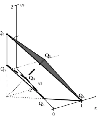
Q4= (0,1,0),Q5= (1,4,0),Q6= (1,0,0).

Their convex hullΓ is a pentahedron (Fig. 12). It has 2D upper faceΓ(2)₁ with external normalN1= (1,0,1)

contain-ing 3 points of the supportS˜: Q1,Q5,Q6. Corresponding

truncated equation is

ˇ

f₁(2)def= −xyy′′+xy′2+cxy4+dx= 0.

It has the first integral

y′2=cy4+C0y2−d def

(9)

[image:9.595.96.267.62.259.2]

Figure 12.3D supporteS(f)and polyhedronΓ(f)of equation (10) with all

a, b, c, d̸= 0. The grey face isΓ(2)₁ . All dotted lines are in the planeq1,

q2, they show projections ofΓ(f)on the plane(q1, q2).

whereC0 ∈ Cis an arbitrary constant. Discriminant of the

polynomialP(y)is∆(P) =−cd(cd+C02/4)2. If∆(P)̸=

0, then solutionsy =φ0(x)of the equation (20) are elliptic

functions. So we can look for expansions (19), where all φl(x)are regular functions ofφ0(x). Hereω = 1andγ1=

0.

5 Partial Differential Equations.

Al-gebraic Approach

5.1

Theory [3]

LetX = (x1, . . . , xm) ∈ Cm be independent andY =

(y1, . . . , yn) ∈ Cn be dependent variables. Suppose Z =

(X, Y)∈Cm+n_{. A}_{differential monomial}_a₍_Z₎_{is the} prod-uct of an ordinary monomialcZR ₌ _czr1

1 · · ·z

rm+n m+n, where c = const∈C,R= (r1, . . . , rm+n)∈Rm+n, and a finite number of derivatives of the form

∂l_y j ∂xl1

1 · · ·∂x

lm m

def

= ∂

l_y j ∂XL,

lj >0, m

∑

j=1

lj =l, L= (l1, . . . , lm).

A differential monomial a(Z) corresponds to its vector

power exponentQ(a)∈Rm+nformed by the following rules Q(cZR) =R, Q(∂lyj/∂XL) = (−L, Ej),

where Ej is unit vector. A product of monomials a· b corresponds to the sum of their vector power exponents: Q(ab) =Q(a) +Q(b).

A differential sum is a sum of differential monomials f(Z) = ∑ak(Z). A setS(f)of vector power exponents Q(ak)is called thesupportof the sumf(Z). The closure of the convex hullΓ(f)of the supportS(f)is called the poly-hedron of the sumf(Z).

Consider a system of equations

fi(X, Y) = 0, i= 1, . . . , n, (21)

wherefiare differential sums. Each equationfi = 0 corre-sponds to: its support S(fi), its polyhedronΓ(fi)with the set of facesΓ(di)

ij in the main spaceRm+n, the set of normal conesU(di)

ij to facesΓ

(di)

ij in the dual spaceR m+n

∗ , and the set of truncated equations

ˆ

f(di)

ij (X, Y) = 0. The set of truncated equations

ˆ

f(di)

iji (X, Y) = 0, i= 1, . . . , n (22) is thetruncated system if the intersection of corresponding normal cones

U(d1)

1j1 ∩ · · · ∩U

(dn)

njn (23)

is not empty. A solutionyi = φi(X),i = 1, . . . , nto sys-tem (21) is associated to its normal coneu⊂Rm+n_{. If the} normal coneuintersects with cone (23), then the asymptotic formyi= ˆφi(X),i= 1, . . . , nof this solution satisfies trun-cated system (22), which is quasi-homogeneous.

5.2

Applications. Boundary layer on a needle [31]

The theory of the boundary layer on a plate for a stream of viscous incompressible fluid was developed by Prandtl (1904) [32] and Blasius (1908) [33]. However a similar the-ory for the boundary layer on a needle was not known until recently, since no-slip conditions on the needle correspond to a more strong singularity as for the plate. This theory was developed with the help of Power Geometry (2004).

Letxbe an axis in three-dimensional real space,rbe the distance from the axis, and semi-infinite needle be placed on the half-axis x> 0,r = 0. We studied stationary axisym-metric flows of viscous fluid which had constant velocity at x = −∞parallel to the axisx, and which satisfied no-slip conditions on the needle (Fig. 13). We considered two cases: (1) incompressible fluid and (2) compressible heat-conducting gas.

0 r

x

[image:9.595.350.514.523.612.2]

u

_∞

Figure 13.The needle and flow along it.

First case: incompressible fluid. For it, the Navier-Stokes equations in independent variablesx,rare equivalent to the system of two equations for the stream functionψand the pressurep

g1 def

= −1

r ∂ψ ∂x

∂ ∂r

( 1

r ∂ψ

∂r

) +1

r ∂ψ

∂r ∂ ∂x

( 1

r ∂ψ

∂r

) +1

ρ ∂p ∂x−

−ν

( 1

r ∂ ∂r

(

r∂ ∂r

( 1

r ∂ψ ∂r

)) + ∂

2

∂x2

( 1

r ∂ψ

∂r

)) = 0,

g2 def

= 1

r ∂ψ ∂x

∂ ∂r

( 1

r ∂ψ ∂x

)

−1

r ∂ψ

∂r ∂ ∂x

( 1

r ∂ψ ∂x

) +1

ρ ∂p ∂r+

+ν

(

∂ ∂r

( 1

r ∂2ψ ∂x∂r

) + ∂

2

∂x2

( 1

r ∂ψ ∂x

)) = 0,

(10)

whereρ, ν= const, with the boundary conditions

ψ=ψ0r2forx=−∞, ψ0= const; (25)

∂ψ/∂x=∂ψ/∂r=∂2ψ/∂x∂r=∂2ψ/∂r2= 0 (26) forx>0,r= 0. Herem=n= 2andm+n= 4.

Hence the supports of equations (24) must be considered in

R4_{. It turned out that polyhedra}_Γ(_g

1)andΓ(g2)of equations

(24) are three-dimensional tetrahedra, which can be moved by translation in one linear three-dimensional subspace, that simplified the isolation of the truncated systems. An analysis of truncated systems and of the results of their matching re-vealed that system (24) had no solution withp>0satisfying both boundary conditions (25), (26).

Second case: compressible heat-conducting gas. For this case, the Navier-Stokes equations in independent vari-ablesx, rare equivalent to the system of three equations for the stream functionψ, the densityρ, and the enthalpyh(an analog of the temperature)

(27) f1

def

= −1

r ∂ψ ∂x ∂ ∂r ( 1 ρr ∂ψ ∂x ) +1 r ∂ψ ∂r ∂ ∂x ( 1 ρr ∂ψ ∂x )

−A ∂

∂r(ρh)

+2 3C N ∂ ∂r ( hN r ∂ ∂r ( 1 ρ ∂ψ ∂x )) −2 3C N ∂ ∂r ( hN r ∂ ∂x ( 1 ρ ∂ψ ∂r ))

−2CN

r ∂ ∂r

(

hNr ∂ ∂r ( 1 ρr ∂ψ ∂x ))

+CN ∂ ∂x

(

hN ∂ ∂r ( 1 ρr ∂ψ ∂r ))

−CN ∂

∂x

(

hN ∂ ∂x ( 1 ρr ∂ψ ∂x ))

+2C

N_hN ρr3

∂ψ ∂x = 0,

(28) f2 def =1 r ∂ψ ∂x ∂ ∂r ( 1 ρr ∂ψ ∂r ) −1 r ∂ψ ∂r ∂ ∂x ( 1 ρr ∂ψ ∂r )

−A ∂

∂x(ρh)

+2 3C N ∂ ∂x ( hN r ∂ ∂r ( 1 ρ ∂ψ ∂x )) −2 3C N ∂ ∂x ( hN r ∂ ∂x ( 1 ρ ∂ψ ∂r )) +C N r ∂ ∂r (

hNr ∂ ∂r ( 1 ρr ∂ψ ∂r ))

−CN

r ∂ ∂r

(

hNr ∂ ∂x ( 1 ρr ∂ψ ∂x ))

+ 2CN ∂ ∂x

(

hN ∂ ∂x ( 1 ρr ∂ψ ∂r )) = 0,

f3 def = 1 r ∂ψ ∂x ∂h ∂r − 1 r ∂ψ ∂r ∂h ∂x − A ρr ∂ψ ∂x

∂(ρh)

∂r

+ A

ρr ∂ψ

∂r ∂(ρh)

∂x + 2C N_hN

( ∂ ∂r ( 1 ρr ∂ψ ∂x ))2

+ 2CNhN

( 1

r2_ρ

∂ψ ∂x

)2

+ 2CNhN

( ∂ ∂x ( 1 ρr ∂ψ ∂r ))2

+CNhN

( ∂ ∂x ( 1 ρr ∂ψ ∂x ))2

−CNhN ∂

∂x ( 1 ρr ∂ψ ∂x ) ∂ ∂r ( 1 ρr ∂ψ ∂r )

+CNhN

( ∂ ∂r ( 1 ρr ∂ψ ∂r ))2 −2 3C

N_hN

( 1 r ∂ ∂r ( 1 ρ ∂ψ ∂x ))2

+4C

N_hN

3r ∂ ∂r ( 1 ρ ∂ψ ∂x ) ∂ ∂x ( 1 ρr ∂ψ ∂r ) −2 3C N hN ( ∂ ∂x ( 1 ρr ∂ψ ∂r ))2 +C N σr ∂ ∂r (

rhN∂h ∂r ) +C N σ ∂ ∂x (

hN∂h ∂x

) = 0,

(29)

where parameters A, C, σ > 0 andN ∈ [0,1], with the boundary conditions

ψ=ψ0r2, ρ=ρ0, h=h0for

x=− ∞, ψ0, ρ0, h0= const

(30)

and (26). Herem= 2,n= 3, andm+n= 5. In the space

R5_{, all polyhedrons}_Γ(_f

1),Γ(f2),Γ(f3)of equations (29) are

three-dimensional, and they can be translated into one linear 3D subspace. In coordinatesQ˜′ = (˜q₁′,q˜₂′,q˜₃′)of this three-dimensional space, the supports and polyhedra are shown in Figures 14–16.

The supports of sumsf1,f2andf3are following:

S(f1) ={Q˜′0= 0,Q˜′1= (1,0,0),Q˜′2= (0,1,0),

˜

Q′₃= (0,0,1)},

S(f2) ={Q˜′0= 0,Q˜′1= (1,−1,1),Q˜′2= (0,1,0),

˜

Q′₃= (0,0,1)},

S(f3) ={Q˜′0= 0,Q˜′1= (0,1,0),Q˜′2= (−1,2,−1),

˜

Q′3= (0,0,1),Q˜′4= (−1,0,1),Q˜′5= (−1,1,0)}.

The truncated system corresponding to the boundary layer on the needle corresponds to the vertex Q˜′₁, to faces

[ ˜Q′0,Q˜′1,Q˜′2]and[ ˜Q′0,Q˜′1,Q˜′2]of polyhedronsΓ(f1),Γ(f2)

(11)

[image:11.595.123.232.66.212.2] [image:11.595.120.235.253.386.2]

Figure 14.The Newton polyhedron off1in (29)

Thus, the truncated system is

ˆ

f₁₂(0)def= −A∂(ρh)/∂r= 0,

ˆ

f₂₂(2)def= 1

r ∂ψ ∂x

∂ ∂r

( 1

ρr ∂ψ ∂r

)

−1

r ∂ψ ∂r

∂ ∂x

( 1

ρr ∂ψ ∂r

)

−

−A ∂

∂x(ρh) + CN

r ∂ ∂r

(

hNr∂ ∂r

( 1

ρr ∂ψ

∂r

)) = 0,

ˆ

f₃₂(2)def= 1

r ∂ψ ∂x

∂h ∂r −

1

r ∂ψ

∂r ∂h ∂x−

A ρr

∂ψ ∂x

∂(ρh)

∂r +

+ A

ρr ∂ψ

∂r ∂(ρh)

∂x +C N_hN

(

∂ ∂r

( 1

ρr ∂ψ

∂r

))2

+

+C

N

σr ∂ ∂r

(

rhN∂h ∂r

) = 0,

(31) with the boundary conditionsψ = ψ0r2,ρ = ρ0,h =h0;

ψ0,ρ0,h0= const, forr→ ∞.

[image:11.595.68.296.455.613.2]

An analysis of solutions to the latter problem (31) by meth-ods of Power Geometry revealed that forN ∈ (0,1) it has

solutions of the form

ψ∼c1r2|logξ|−1/N, ρ∼c2|logξ|−1/N, h∼c3|logξ|1/N,

(32) whereξ = r2/x → 0 andc1, c2, c3 are arbitrary real

con-stants. Thus, forN ∈(0,1), in the boundary layerr2_{/x <}

const, asx → +∞ andξ = r2_/x _→ ₀_{, we obtained the}

asymptotic form of the flow (32), i.e. near the needle, the densityρtends to zero, and the temperaturehincreases to in-finity as the distancexto the initial point of the needle tends to+∞.

5.3

Other applications of Power Geometry

Evolution of the turbulent flow [34, 35] and Thermody-namics [36] and power-elliptic expansions of solutions to Painlev´e equations [37].

6 Connection with Idempotent

Math-ematics

For polynomialf(X), let us define the function

ˆ

f(S) = lim

h→+0hlog|f(exp(S/h))|

and itssubdifferential

∂fˆ={Q∈Rn:⟨Q, S⟩6fˆ(S)for allS∈Rn_∗}.

Theorem 6 ( [38]) Iff(X)is a polynomial, then the subdif-ferential∂fˆoff(X)at the origin coincides with the Newton polyhedronΓ(f).

V. P. Maslov and his colleagues developed Idempotent Analysis [38, 39]. However, as a method of finding leading terms in nonlinear problems, it is too complicated. Theo-rem 6 shows that in algebraic problems Idempotent Analy-sis gives the Newton polyhedron. This observation can be generalized to other classes of problems, but if we just be-gin with appropriate generalization of the Newton polyhe-dron (or Power Geometry), then we do not really need Idem-potent Analysis (see Sections 4 and 5). Indeed, IdemIdem-potent Analysis [39] is useful in problems with “bad” solutions (for instance, discontinuous or non-smooth).

REFERENCES

[1] Bruno, A.D.: The asymptotic behavior of solutions of nonlinear systems of differential equations. DAN SSSR

143:4, 763–766 (1962) (in Russian). English transla-tion: Soviet Math. Dokl.3464–467 (1962)

[2] Bruno, A.D.: Local Methods in Nonlinear Differential Equations. Moscow, Nauka (1979) (in Russian). En-glish translation: Springer–Verlag, Berlin–New York (1989)

(12)

[4] Bruno, A.D., Batkhin, A.B.: Asymptotic solu-tion of an algebraic equasolu-tion. DAN 440:3 , 295– 300 (2011). English translation: Doklady Mathemat-ics 84:2, 634–639 (2011) http://dx.doi.org/10.

1134/S1064562411060160.

[5] Newton, I.: The Method of Fluxions and Infinite Series with its Applications to the Geometry of Curve Lines. New York; London, Johnson Reprint Corp. (1964) [6] Briot, C., Bouquet, T.: Recherches sur les propri´et´es

des ´equations differentielles. J. Ecole Polytechn. Paris,

21, No 36 (1856).

[7] Mikhailov, V.P.: On the first boundary value problem for some semi-bounded operators. Dokl. Akad. Nauk SSSR,151, 282–285 (1963) (in Russian). English trans-lation: Sov. Math. Dokl.4, 997–1001 (1963)

[8] Bruno, A.D.: On geometric methods in works by V.I. Arnold and V.V. Kozlov. Preprint ArXiv: 1401.6320v1.

[9] Bruno, A.D., Batkhin, A.B.: Resolution of algebraic singularity by algorithms of Power Geometry. Pro-grammirovanie. 38:2, 12–30 (2012) (in Russian). En-glish translation: Programming and Computer Soft-ware. 38:2, 57–72 (2012) http://dx.doi.org/10.

1134/S036176881202003X.

[10] Batkhin, A.B., Bruno, A.D., Varin, V.P.: Sets of stability of multiparameter Hamiltonian systems. PMM. 76:1, 80–133 (2012) (in Russian). English translation: J. Appl. Math. Mech.76:1, 56–92 (2012)

http://dx.doi.org/10.1016/j.jappmathmech.

2012.03.006.

[11] Bruno, A.D.: Asymptotics and expansions of solutions to an ordinary differential equation. UMN. 59:3, 31– 80 (2004) (in Russian). English translation: Russian Mathem. Surveys.59:3, 429–480 (2004)http://dx.

doi.org/10.1070/RM2004v059n03ABEH000736.

[12] Bruno, A.D., Goryuchkina, I.V.: Asymptotic expan-sions of solutions of the sixth Painlev´e equation. Trudy Mosk. Mat.Obs. 71, 6–118 (2010) (in Russian). En-glish translation: Transactions of Moscow Math. Soc.

71, 1–104 (2010) http://dx.doi.org/10.1090/

S0077-1554-2010-00186-0.

[13] Bruno, A.D., Goryuchkina, I.V.: All expansions of solutions to the sixth Painlev´e equation near its non-singular point. Doklady Akademii Nauk. 426:5, 586– 591 (2009) (in Russian). English translation: Doklady Mathematics.79:3, 397–402 (2009)http://dx.doi.

org/10.1134/S1064562409030260.

[14] Bruno, A.D.: Power asymptotics of solutions to an ODE system. DAN. 410:5, 583–586 (2006) (in Russian). English translation: Doklady Mathemat-ics. 74:2, 712–715 (2006) http://dx.doi.org/10.

1134/S1064562406050243.

[15] Bruno, A.D.: Power-logarithmic expansions of solutions to a system of ordinary differen-tial equations. DAN. 419:3, 298–302 (2008) (in Russian). English translation: Doklady

Mathematics. 77:2, 215–218 (2008) http: //dx.doi.org/10.1134/S1064562408020154

[16] Bruno, A.D.: Nonpower asymptotic forms of solutions to a system of ordinary differential equations. DAN.

420:1, 7–10 (2008) (in Russian). English translation: Doklady Mathematics. 77:3, 325–328 (2008) http:

//dx.doi.org/10.1134/S1064562408030010.

[17] Bruno, A.D.: Complicated expansions of solutions to a system of ordinary differential equations. DAN.421:1, 7–10 (2008) (in Russian). English translation: Doklady Mathematics.78:1, 477–480 (2008)http://dx.doi.

org/10.1134/S1064562408040017.

[18] Bruno, A.D., Parusnikova, A.V.: Local expansions of solutions to the fifth Painlev´e equation. 438:4, 439– 443 (2011) (in Russian). English translation: Doklady Mathematics.83:3, 348–352 (2011)http://dx.doi.

org/10.1134/S1064562411030276.

[19] Bruno, A.D., Parusnikova, A.V.: Expansions of so-lutions to the fifth Painlev´e equation near its non-singular point. DAN, 442:5, 583–588 (2012) (in Russian). English translation: Doklady Mathematics.

85:1, 87–92 (2012) http://dx.doi.org/10.1134/ S1064562412010292

[20] Bruno, A.D.: Families of periodic solutions to the Beletsky equation. Kosmicheskie Issledovanija. 40:3, 295–316 (2002) (in Russian). English translation: Cos-mic Research.40:3, 274–295 (2002)

[21] Bruno, A.D.: Analysis of the Euler-Poisson equa-tions by methods of Power Geometry and Nor-mal Form. PMM. 71:2, 192–227 (2007) (in Rus-sian). English translation: J. Appl. Math. Mech.71:2, 168–199 (2007) http://dx.doi.org/10.1016/j.

jappmathmech.2007.06.002.

[22] Bruno, A.D., Varin, V.P.: Periodic solutions of the restricted three-body problem for small mass ra-tio. PMM .71:6, 1034–1066 (2007) (in Russian). English translation: J. Appl. Math. Mech. 71:6, 933–960 (2007) http://dx.doi.org/10.1016/j. jappmathmech.2007.12.012

[23] Bruno, A.D., Varin, V.P.: On asteroid distribu-tion. Astronomicheskii Vestnik.45:4, 334–340 (2011) (in Russian). English translation: Solar System Re-search.45:4, 323–329 (2011) http://dx.doi.org/

10.1134/S0038094611040010.

[24] Bruno, A.D., Edneral, V.F.: Algorithmic analysis of local integrability. DAN. 424:3, 299–303 (2009) (in Russian). English translation: Doklady Mathematics.

79:1, 48–52 (2009) http://dx.doi.org/10.1134/ S1064562409010141

[25] Bruno, A.D.: Space Power Geometry for an ODE and Painleve equations.In: International Conference ”Painleve Equations and Related Topics”. pp. 36–41. St. Petersburg, June, (2011)

(13)

137–142 (2012) (in Russian). English translation: Dok-lady Mathematics.85:3, 336–340 (2012)http://dx.

doi.org/10.1134/S106456241203009X.

[27] Bruno, A.D.: Space Power Geometry for an ODE and P1–P4, P6. In: Bruno, A.D., Batkhin, A.B. (eds.)

Painlev´e Equations and Related Topics, pp. 41–51. De Gruyter, Berlin/Boston (2012)

[28] Bruno, A.D., Parusnikova, A.V.: Elliptic and periodic asymptotic forms of solutions toP5. In: Bruno, A.D.,

Batkhin, A.B. (eds.) Painlev´e Equations and Related Topics (Eds. A.D. Bruno and A.B. Batkhin), pp. 53–65. De Gruyter, Berlin/Boston (2012)

[29] Bruno, A.D.: Regular asymptotic expansions of solu-tions to one ODE and P1–P5. Bruno, A.D., Batkhin,

A.B. (eds.) Painlev´e Equations and Related Topics (Eds. A.D. Bruno and A.B. Batkhin), pp. 67–82. De Gruyter, Berlin/Boston (2012)

[30] Bruno, A.D.: Power-elliptic expansions of solu-tions to an ODE. Zhurnal Vychisl. Matem. i Matem. Fiziki. 52:12, 2206-2218 (2012) (in Russian). En-glish translation: Comp. Mathem. Math. Phys. 52:12, 1650-1661 (2012) http://dx.doi.org/10.1134/

S0965542512120056.

[31] Bruno, A.D., Shadrina, T.V.: Axisymmetric bound-ary layer on a needle. Trudy Mosk. Mat. Ob-sch. 68. 224–287 (2007) (in Russian). English translation: Transactions of Moscow Math. Soc.

68, 201–259 (2007) http://dx.doi.org/10.1090/

S0077-1554-07-00165-3.

[32] Prandtl, L.: ¨Uber Fl¨ussigkeitsbewegung bei sehr kleiner Reibung. In: Verhandl. III Kongr., Heidelberg (1904)

[33] Blasius, H.: Grenzschichten in Fl¨ussigkeiten mit kleiner Reibung. Zeit. f¨ur Math. und Phys. 56, 1–37 (1908)

[34] Bruno, A.D.: Power geometry in nonlinear partial dif-ferential equations. Ukrainean Mathem. Bulletin.5:1, 32–45 (2008)

[35] Bruno, A.D.: Power geometry in differential equa-tions. “Contemporary Problems of Mathematics and Mechanics”. Mathematics. Dynamical Systems. MGU. Moscow,4:2, 24–54 (2009) (in Russian)

[36] Bruno, A.D.: Self-similar solutions and Power Ge-ometry. Uspekhi Mat. Nauk. 55:1, 3–44 (2000) (in Russian). English translation: Russian Math. Surveys,

55:1, 1–42 (2000) http://dx.doi.org/10.1070/

RM2000v055n01ABEH000248.

[37] Bruno, A.D.: Power geometry and elliptic expansions of solutions to the Painlev´e equations. International Journal of Differential Equations, V. 2015. Article ID 340715, 13 phttp://dx.doi.org/10.1155/2015/ 340715.

[38] Litvinov, G.L., Shpiz, G.B.: The dequantization trans-form and generalized Newton polytopes. In: Litvinov, G.L., Maslov, V.P. (eds.) Idempotent Mathematics and Mathematical Physics. pp. 99-104. Contemporary Mathematics, 377, AMS, Providence, RI (2005) [39] Maslov, V.P., Kolokoltsov, V.N.: Idempotent