Impulsive differential equations by using the Euler method

Impulsive Differential Equations

by using the Euler Method

Nor Shamsidah Bt Amir Hamzah1, Mustafa bin Mamat2 , J. Kavikumar3, Lee Siaw Chong4 and Noor’ani Bt Ahmad5

1, 2, 5

Department of Mathematics, Faculty of Science and Technology Universiti Malaysia Terengganu, 21030 Kuala Terengganu, Terengganu, Malaysia

[email protected] (Mustafa bin Mamat)

3,4

Department of Science and Mathematics, Faculty of Science, Arts and Heritage Universiti Tun Hussein Onn Malaysia, 86400 Parit Raja, Johor, Malaysia

Abstract

The theory of impulsive differential equations is emerging as an important area of investigation since such equations appear to represent a natural framework for mathematical modeling of several real phenomena. There have been intensive studies on the qualitative behavior of solutions of the impulsive differential equations. However, many impulsive differential equations cannot be solved analytically or their solving is complicated. In this paper, we represent the algorithm which follows the theory of impulsive differential equations to solve the impulsive differential equations by using the Euler methods. It is clearly shown the impulsive operators Ik that acts

at the moments t_k influence the error. Finally, the better convergence result of the numerical solution is given by solving the numerical examples.

Keywords: Differential Equations, Impulsive Differential Equations, Fixed impulse, Impulsive jump, Euler Method

1.

Introduction

process. It is assume naturally, that those perturbations act instantaneously, in the form of impulses. Thus impulsive differential equations, by means, differential equations involving impulse effects, are seen as a natural description of observed evolution phenomenon of several real world problems. For example, mechanical system with impact, biological phenomenon involving thresholds, bursting rhythm models in medicine and biology, optimal control models in economics, pharmacokinetics and industrial robotics, and many more, do exhibit impulsive effects. Therefore, it is beneficial to study the theory of impulsive differential equations as a well deserved discipline, due to the increase applications of impulsive differential equations in various fields in the future. The pioneer papers in this theory are written by A. D. Myshkis and V. D. Mil’man in 1960’s [9].

In spite of its importance, many solutions regarded to impulsive differential equations are done analytically. Some of the famous researchers who presented significance results are V. Lakshmikantham, D. Bainov, P. Simeonov and many others [ 1, 3, 4, 5, 6, 7, 8, 10 ]. However, many impulsive differential equations cannot be solved analytically or if done, their solving is very much complicated [11]. Therefore, numerical solutions of impulsive differential equations has to be studied and the results has to be improved. In this paper, the numerical solutions of impulsive differential equations are sought by using the Euler method. The algorithm proposed is interpreted according to the theory of impulsive differential equations written by V. Lakshmikantham et. al [8]. Based on the theory, the better numerical solution of the problem is illustrated in the examples.

2.

Impulsive Differential Equations

Basically, impulsive differential equations consist of three components.

A continuous-time differential equation, which governs the state of the system between impulses, an impulse equation, which models an impulsive jump, defined by a jump function at the instant an impulse occurs, and a jump criterion, which defines a set of jump events. Mathematically, the equation takes the form,

m k

t x I t x

Z t t t x t f t x

k k k

k

,..., 2 , 1 )),

( ( ) (

, ),

, ( ) ( '

= =

Δ

∈ ≠

=

(2.1)

where Z is any real interval, f :Z×Rn →Rn is a given function,

m k

R R

Ik : n → n, =1,2,..., and Δx(tk)=x(tk )−x(tk ),k =1,2,...,m.

− +

The numbers

k

t are called instants (or moments) of impulse, Ik represents the jump of state at each

k

on the state of the system. In this paper, we will be concerned with fixed moments only.

Moreover, impulsive differential equations can be classified according to these three components.

1. Systems with impulse at fixed moments. The equations have the following

form

k k

k

t t x I x

t t x t f t x

= =

Δ

≠ =

), (

, ),

, ( ) ( '

(2.2)

where t₀ <t₁<...<t_k <t_k+1<..., k∈Z and for t =t_k, Δx(t_k)=x(t_k+)−x(t_k−)

where ( ) lim ( )

0 x t h

t

x k

h

k = _→ + +

+

. We surely see that any solution, x(t) of (2.2) satisfies

(i) x'(t)= f(t,x(t)), t∈(tk,tk+1) and (ii) Δx(tk)=Ik(x(tk)), t=tk, k=1,2,...

2. Systems with impulse at variable times. The equations have the following

form

... , 2 , 1 ),

( ),

(

), ( ),

, ( ) ( '

= =

= Δ

≠ =

k x t

x I x

x t

x t f t x

k k

k

τ τ

(2.3)

where τ_k =Ω→R, Ω is the phase space, and τk(x)<τk+₁(x), k∈Z, x∈Ω.

Systems with variable moments of impulsive effect involve more difficult problems than systems with fixed moments of impulsive effect. This is due to the fact that the moments of impulsive effect of (2.3) depend on the solution, i.e. t =τk(x), for each k. Therefore, solutions at different starting points will have different points of discontinuity.

3. Autonomous systems with impulse. The equations take the form

M x x

I x

M x x

f t x

∈ =

Δ

∉ =

), (

, ),

( ) ( '

(2.4)

Let the sets M(t) = M, N(t) = N and the operator A(t) = A be independent of t and

) , 0 , ( )

(t x t x0

x = hits the set M at some time t, the operator A instantly transfers the

point x(t)∈M into the point y(t)=x(t)+I(x(t))∈N.

Generally, the solutions of the impulsive differential equations are piecewise continuous functions with points of discontinuity at the moments of the impulse effect.

In this paper, we denote S ={tk :k∈Z}⊂R where tk <tk+1 for all

∞ + → ∈Z t_k

k , when k →+∞ and t_k →−∞ when k →−∞. If Ω⊂ Ris any

real interval, we suppose that x(t)=[x1(t)

T n t

x t

x2( ) ... ( )] , is a vector of

unknown functions, and

f :Ω×Rn →Rn,

⎥ ⎥ ⎥ ⎥ ⎥ ⎥

⎦ ⎤

⎢ ⎢ ⎢ ⎢ ⎢ ⎢

⎣ ⎡

=

) ( ..., ), ( ), ( , (

... ...

...

... ...

...

) ( ..., ), ( ), ( , (

) ( ..., ), ( ), ( , (

) , (

2 1

2 1 2

2 1 1

t x t

x t x t f

t x t x t x t f

t x t x t x t f

x t f

n n

n n

is continuous function on every set [tk,tk+1]×Rn.

Definition 2.1

A system of differential equation of the form

k

t t x t f dt

dx_{= ≠}

), ,

( (2.5)

with conditions

)) ( ( ) ( ) (

|_{t t} x t_k x t_k I_k x t_k

x

k= − =

Δ + −

=

where Ik :Rn →Rn are continuous operators, k =0,±1,±2,... is called impulsive

3.

Properties of Solutions of IDEs

The problem of existence and uniqueness of the solutions of impulsive differential equations is similar to that of corresponding ordinary differential equations. The continuability of solutions is affected by the nature of the impulsive action.

Definition 3.1

A solution of the IDE (2.5) means a piecewise continuous x:J →Rwith

piecewise continuous first derivative such that

1. f t x t t k

dt t

dx _{= ≠τ}

)), ( , ( ) (

2. x(τk+)−x(τk−)=Ik(x(τk)), k=0,±1,±2,...

Theorem 3.1

Let the function n

R R

f : ×Ω→ be continuous on the sets

Z k

k

k, +]×Ω, ∈

(τ τ ₁ and for each k∈Z and x∈Ω, suppose there exists the finite

limit of f(t,x) as (t, y)→(τ_k, x), t>τ_k. Then, for each (t0,x0)∈R×Ω, there exists T >t₀ and a solution x:(t₀,T)→Rn of the problem (2.5) with initial condition x(t₀+)=x₀. Furthermore, if the function f is locally Lipschitz continuous with respect to x in R×Ω, then this solution is unique.

Let x(t) be the solution of IDE (2.5) with initial condition x(t0 )=x0 +

, then x(t) can be represented as

⎪ ⎪ ⎩ ⎪ ⎪ ⎨ ⎧

Ω ∈ −

+

Ω ∈ +

+ =

∑

∫

∑

∫

< <

− <

<

+

t t t

k k t

t

t t t

k k t

t

k k

t t

x I ds

s x s f x

t t

x I ds

s x s f x

t x

0 0

0 0

, )) ( ( ))

( , (

, )) ( ( ))

( , (

) (

0 0

Theorem 3.2

Assume that f ∈C[I×En,En] and satisfies, d[f(t,u), f(t,v)]≤Ld[u,v], L>0 for

n

E I v t u

t, ),(, )∈ ×

( . Then the initial value problem (2.5) has a unique solution

) , , ( )

(t u t t0 u0

u = on I.

We also need the following known [8] impulsive differential inequalities result. For

this purpose, we let PC denote the class of piecewise continuous functions from R+

to Rwith discontinuous of the first kind only at t=tk;k =1,2,...We can now state the

needed results.

Theorem 3.3

Assume that )

(A0 the sequence {tk}satisfies 0≤t0 <t1<t2 <K<tk <Kwith tk →∞as k→∞;

)

(A₁ m∈PC'[R₊,R]and m(t)is left continuous at t_k,k =1,2,...

)

(A2 ∀k =1,2,Kand t ≥t0

⎢ ⎢ ⎢

⎣ ⎡

≤ ≤

≠ ≤

+ +

0

0)

(

)), ( ( ) (

, )),

( , ( ) (

w t m

t m t

m

t t t m t g t m D

k k k

k

ψ (3.1)

where g:R+2 →Ris continuous in (tk−1,tk]×R+and for each w∈R+,

lim (, ) ( , )

) , ( ) ,

(tz tk w g t z g tk w

+

→ + = exists and ψk :R+ →Ris non-decreasing;

)

(A3 r(t)=r(t,t0,w0)is the maximal solution of

⎢ ⎢ ⎢

⎣ ⎡

≥ =

=

≠ =

′

+

0 )

(

)), ( ( ) (

), , (

0

0 w

t w

t w t

w

t t w

t g w

k k k

k

ψ (3.2)

existing on [t0,∞). Then

m(t)≤r(t), t≥t0 (3.3)

⎢ ⎢ ⎢ ⎢ ⎢ ⎢ ⎢ ⎢ ⎢ ⎢

⎣ ⎡

∈ ∈ ∈

= − + +

+

M M M

] ( )) ( , , (

] ( )),

( , , (

] [ ),

, , (

)

( _{1 , 1}

2 , 1 1

0 1 1

1 , 0 0

0 0

k k k

k k

k t t r t t t t

r

t t t t

r t t r

t t t w

t t r

t

r (3.4)

where each r_i(t,t_i,r_i−1(t_i+))is the maximal solution of (2.3) on the interval (t_i,t_i+1] for each i=1,2,_K, and r_i−1(t_i+)=ψ_i(r_i−1(t_i,t_i−1,r_i−2(t_i+₋₁))).

4.

Algorithm

Suppose the IDE (2.5) with start condition x₀ =x(t₀)and the impulsive operators

) (

, k Z

Ik ∈ is given. The impulsive operators act at the moments of jump happen, tk

for all k∈Z which are described by the quadrate matrices of dimensions n×n.

The numerical algorithm is different only at the jump point, where we have to apply the operators concern with the particular point. Other than that, we employ the usual manners to solve the IDE using the numerical method chosen.

1. At the moment, t=t0, we apply the numerical method to the function with the

initial values x=x₀. The algorithm applies until the first jump point, by now we will get the values for the left limit.

2. At the jump point, t =tk, we apply the operators to find the values of the right

limit.

3. The first step is repeated until the next jump point.

4. Then, we apply the operators concern with the particular jump point.

5. The above steps are repeated and the iteration stop until we encounter with the

desired values that has to be found, let assume, ts where ts >t0. Notice that we only have the approximate values of the function at t =ts.

5.

Numerical Examples

k t t x t f dt

dx _{= ≠}

), , (

Δx(tk)=Ik(x(tk)), t=tk, k=1,2,... (5.1)

) ( 0

0 x t

x =

and t₀ =0.0,

⎥ ⎦ ⎤ ⎢ ⎣ ⎡− = ⎥ ⎦ ⎤ ⎢ ⎣ ⎡ = 0 1 , ) ( ) ( 0 2 1 x t x t x x ⎥ ⎦ ⎤ ⎢ ⎣ ⎡ + − − + + = 5833333 . 0 1666666 . 0 1666666 . 0 1666666 . 0 1666666 . 0 1666666 . 0 ) , ( 2 1 2 1 x x x x x t f

The impulsive operators act at t1 =1.0 and t2 =2.0 are given as follows:

⎥ ⎦ ⎤ ⎢ ⎣ ⎡ − = ⎥ ⎦ ⎤ ⎢ ⎣ ⎡ − = 0 . 1 0 . 0 0 . 4 0 . 3 , 0 . 1 0 . 0 25 . 0 25 . 0 2 1 I

I (5.2)

Here, we wish to approximate the value of t_s =2.3. We applied the algorithm by using the Euler method,

xi+1 =xi +hf(t, xi) (5.3)

where i∈Z is the index of iteration, and h is the step size of each iteration. Here, the step size h = 0.1. Then we compared the results obtained by using the analytical expression that is the solution of IDE (5.1).

⎪ ⎪ ⎪ ⎪ ⎪ ⎩ ⎪⎪ ⎪ ⎪ ⎪ ⎨ ⎧ ∞ ∈ − + − = ∞ ∈ − = ∈ − + − = ∈ − = −∞ ∈ + − = −∞ ∈ − = = ) , 2 [ , 25 . 1 75 . 0 0625 . 0 ) ( ) , 2 [ , 25 . 1 0625 . 0 ) ( ) 2 , 1 [ , 6875 . 0 75 . 0 0625 . 0 ) ( ) 2 , 1 [ , 0625 . 1 0625 . 0 ) ( ) 1 , ( , 75 . 0 0625 . 0 ) ( ) 1 , ( , 0 . 1 0625 . 0 ) ( 2 2 2 1 2 2 2 1 2 2 2 1 t t t t x t t t x t t t t x t t t x t t t t x t t t x

x (5.4)

Table 1 : The approximate values at t = 2.3

k

t Euler

) (

1 tk

x

Analytical ) (

1 tk

x

Euler ) (

2 tk

x

Analytical ) (

2 tk

x 0.0

0.1 0.2 0.3 0.4 0.5 0.6 0.7 0.8 0.9 1.0

-1 -1 -0.9988 -0.9963 -0.9925 -0.9875 -0.9813 -0.9738 -0.965 -0.955 -0.9438

-1.0 -0.9994 -0.9975 -0.9944 -0.9900 -0.9844 -0.9775 -0.9694 -0.9600 -0.9494 -0.9375

0 0.075 0.1487 0.2212 0.2925 0.3625 0.4312 0.4987 0.565 0.63 0.6937

0.0 0.0744 0.1475 0.2194 0.2900 0.3594 0.4275 0.4943 0.5600 0.6244 0.6875 1.0

1.1 1.2 1.3 1.4 1.5 1.6 1.7 1.8 1.9 2.0

-1.0063 -1.0064 -1.0052 -1.0028 -0.9992 -0.9943 -0.9881 -0.9807 -0.9721 -0.9622 -0.9510

-1.0 -0.9869 -0.9725 -0.9569 -0.9449 -0.9219 -0.9025 -0.8819 -0.8600 -0.8369 -0.8125

0.0 0.0751 0.149 0.2216 0.2929 0.363 0.4319 0.4995 0.5658 0.6309 0.6948

0.0 0.06 0.1225 0.1819 0.2468 0.2969 0.3525 0.4069 0.4600 0.5119 0.5625 2.0

2.1 2.2 2.3

-1.0250 -1.0254 -1.0246 -1.0225

-1.0 -0.9744 -0.9475 -0.9193

0.0 0.0754 0.1496 0.2225

0.0 0.0549 0.0975 0.1444

-1.2 -1 -0.8 -0.6 -0.4 -0.2 0

t

x1

Figure 1 The approximate values of x1 versus time, t between the euler and analytical method for Example 1

0 0.1 0.2 0.3 0.4 0.5 0.6 0.7 0.8

0

t

x2

Example 2 Consider the IDE, k t t x t f dt dx ≠ = (, ),

Δx(t_k)=I_k(x(t_k)), t=t_k, k=1,2,... (5.5)

) ( 0

0 x t

x =

and t0 =0.0,

⎥ ⎦ ⎤ ⎢ ⎣ ⎡ − = ⎥ ⎦ ⎤ ⎢ ⎣ ⎡ = 2 2 , ) ( ) ( 0 2 1 x t x t x x , ⎥ ⎦ ⎤ ⎢ ⎣ ⎡ − − = 1 2 1 2 ) , ( x x x x t f

At k = 1, _⎥

⎦ ⎤ ⎢ ⎣ ⎡ − = 8020 . 0 0000 . 0 6565 . 3 0000 . 1 k

I . Here, we wish to determine the approximate

value at t = 1.

For that purpose we apply the Euler method (5.3). Then we compared the results obtained by using the analytical expression that is the solution of IDE (5.1).

⎪ ⎪ ⎪ ⎪ ⎪ ⎪ ⎩ ⎪ ⎪ ⎪ ⎪ ⎪ ⎪ ⎨ ⎧ + − − = ∈ − + − = − − = ∈ + − = = − − − − 0980 . 8 3 4 3 2 ) ( ] 2 , 1 ( 4619 . 17 3 8 3 2 ) ( 3 4 3 2 ) ( ] 1 , 0 ( 3 8 3 2 ) ( 2 2 2 1 2 2 2 1 t t t t t t t t e e t x t e e t x e e t x t e e t x

Table 2 : The approximate values at t = 1.

k

t Euler

) (

1 tk

x

Analytical ) (

1 tk

x

Euler ) (

2 tk

x

Analytical ) (

2 tk

x 0.0

0.1 0.2 0.3 0.4 0.5 0.6 0.7 0.8 0.9 1.0

2.0000 2.6000 3.3000 4.1220 5.0922 6.2419 7.6083 9.2363 11.1792 13.5011 16.2788

2.0000 2.6538 3.4324 4.3651 5.4879 6.8444 8.4878 10.4828 12.9085 15.8614 19.4589

-2.0000 -2.2000 -2.4600 -2.7900 -3.2022 -3.7114 -4.3356 -5.0964 -6.0201 -7.1380 -8.4881

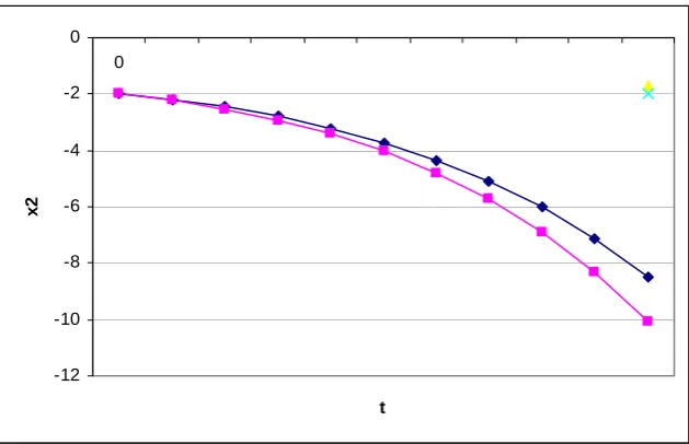
-2.0000 -2.2318 -2.5349 -2.9234 -3.4143 -4.0287 -4.7927 -5.7380 -6.9036 -8.3372 -10.0973

1.0 1.5209 1.9970 -1.6806 -1.9993

0.4761 0.3187

0 5 10 15 20 25

0

t

x1

-12 -10 -8 -6 -4 -2 0

0

t

x2

Figure 4 The approximate values of x2 versus time, t between the euler and analytical method for Example 2

Here, the impulsive operators Ik that acts at the moments tk also influence the

error. This is due to our calculation of the approximate values of the jumps only.

6. Concluding remarks

The accuracy of the results can be improved by investigating the solutions of the other numerical methods. We proposed a general numerical procedure for treating the impulsive differential equations at fixed moments. We interpreted the numerical algorithm following the theory of impulsive differential equations and

started with the Euler method. Although it is not the most accurate methods we will

study, it is by far the simplest, and analyzing Euler’s method in detail will hopefully carries over to the other methods with higher accuracy without a lot of difficulty. Solving the impulsive differential equations numerically has not been done by many researchers. Therefore, many studies have to be done in order to enhance and verify the existing results. In this paper, we have shown better results with diagrams to the convergence and the behavior of the solutions.

References

[1] A. M. Samailenko, N.A. Perestyuk, Impulsive Differential Equations, World Scientific, Singapore, 1995.

[2] B. M. Randelovic, L. V. Stefanovic, B. M. Dankovic, Numerical solution of impulsive differential equations, Facta Univ. Ser Math. Inform, 15 (2000), 101 – 111.

[3] D. D. Bainov, G. Kulev, Application of Lyapunov’s functions to the investigation of global stability of solutions of systems with impulses, Appl. Anal., 26 (1) (1988), 255 – 270.

[4] D. D. Bainov, P.S. Simenov, Systems with Impulse Effect Stability Theory and Applications. Ellis Horwood Limited, Chichester, 1989.

[5] D. D. Bainov, S. I. Kostadinov, N. van Minh, P. P. Zabreiko, A topological

classification of differential equations with impulse effect, Tamkang J. Math. 25 (1994), 15 - 27.

[6] G. Kulev D. D. Bainov, On the stability of systems with impulsive by direct method of Lyapunov, J. Math. Anal. Appl., 140 (1989), 324 – 340.

[7] M. U. Akhmetov, A. Zafer, Successive approximation method for quasilinear impulsive differential equations with control, Appl. Math. Lett., 13 (2000), 99 – 105.

[8] S. Jianhua, New maximum principles for first order impulsive boundary value problems, Appl. Math. Lett, 16 (2003), 105 – 112.

[9] V. D.Mil’man, A. D. Myshkis, On the stability of motion in the presence of impulses, Sib. Math J., 1 (1960), 233-237.

[10] V. Lakshmikantham, D. D. Bainov, P. S. Simeonov, Theory of Impulsive Differential Equations, World Scientific, Singapore, New Jersey, London, Hong Kong, 1989.

[11] X. J. Ran, M. Z. Liu, Q. Y. Zhu, Numerical methods for impulsive differential equation, Mathematical and Computer Modelling, 48 (2008), 46 – 55.