5685
Q-LEARNING WITH ADAPTIVE KANERVA CODING ON
PROTEIN DOCKING
1ERZAM MARLISAH, 1RAZALI YAAKOB, 1MD NASIR SULAIMAN, 2MOHD BASYARUDDIN
ABDUL RAHMAN
1Faculty of Computer Science and Information Technology, University Putra Malaysia, 43400 UPM
Serdang, Selangor, Malaysia
2Faculty of Science, University Putra Malaysia, 43400 UPM Serdang, Selangor, Malaysia
E-mail: 1{erzam, razaliy, nasir}@upm.edu.my 2[email protected]
ABSTRACT
Molecular docking is an important process in pharmaceutical research and drug design. It is used in screening libraries of small molecules or ligands to bind to a target protein changing its original biochemical properties forming new stable complex. In docking ligand to protein, the ligand’s pose, i.e. position, orientation and torsion angles, is translated, orientated, and the ligand’s torsion angles are rotated repeatedly to find an ideal site on the protein to bind. In this paper, Q-learning algorithm, a model-free reinforcement learning, with adaptive Kanerva Coding is used as the searching algorithm for protein-ligand docking problem. It evaluates the effectiveness of Q-learning algorithm and the different settings for the parameters of reinforcement learning. A popular docking tool called AutoDock Vina was used to find the ligand’s goal pose. The effectiveness of the agent is measured by the success of finding the goals. The proposed agent managed to match and finds better pose than AutoDock Vina in medium to large size ligands.
Keywords: Reinforcement Learning, Q-learning, Protein-Ligand Docking, Machine Learning, Kanerva
Coding
1. INTRODUCTION
The chemical property of a lead compound (receptor) can be modified by binding it with smaller molecule (ligand). This process is preceded with computer simulation to predict the resulting complex structure. It involves positioning the ligand, orientating it and twisting its torsion angles relative to the receptor’s binding site. The ligand’s current position, orientation and torsion angle at any moment is called the ligand’s pose. As they are many possible poses, they are ranked according to an energy function calculated by summing up the interaction energy between all pairs of atoms that can move relative to each other. Protein docking problem is then an optimization problem involving the position, orientation and torsion angles aims in minimizing the energy of the complex. Docking ligands with high number of rotatable bonds will be difficult as the number of dimensions becomes larger resulting in poor structure with high binding energy. AutoDock Vina (Vina), a popular molecular docking software, uses Broyden-Fletcher-Goldfarb-Shanno (BFGS) algorithm in
optimizing the ligand’s pose. Its ability to dock highly flexible ligands decreases as the Hessian matrix needed to guide its search becomes larger due to the high dimensions.
5686 effect of the agent’s various parameters and the second part is to determine the agent’s effectiveness. Finally, section 5 concludes the paper and shows direction for future work.
2. RELATED WORK
Prior work in search algorithm for protein-ligand docking has been, among others, is to use modified genetic algorithm, particle swarm optimization and Monte Carlo method. Genetic algorithm has been reported of having decreasing performance in docking ligands with high number of rotatable bonds. This is due to the genetic algorithm encountered premature convergence and stuck in local optimum. Some works combine these methods with local search operator such Solis and Wets algorithm [2] and quasi newton method such as Swarm Optimization for Highly Flexible Protein-Ligand Docking or SODOCK [3] and Lamarckian Genetic Algorithm (LGA) [4]. Solis and Wet algorithm uses distribution of past solutions to select next solution. Unlike the quasi-newton method, it does not exploit any gradient information. More recent methods such as PSOVina, ALPS and VINA were reported to find better conformation [5][6][7]. ALPS extends AutoDock program by applying genetic algorithm with an age property associated with each individual in its population and generate new individuals to guarantee diverse population. In the newer version of AutoDock, the AutoDock Vina , BFGS algorithm is implemented as local search after random mutations of the ligand’s current pose. The mutated individual is then subjected to Metropolis acceptance rule. BFGS finds the next better pose not only by the value of the scoring function but also by calculating the searching direction using approximation of Hessian matrix and the gradient information of the scoring function. PSOVina uses particle swarm optimization technique to replace Vina’s global optimization algorithm and combine it with BFGS. However, protein docking problem is a challenging optimization task due to the energy landscape of all possible conformations is non-convex with rugged and funnel shape [8][9]. A misfit of 0.24A in the average contacts between charged groups of the ligand and the binding area inherently decreases the ligand efficiency by at least 0.1 kcal/mol-atom [10]. A potential ligand could be disregarded due to inaccuracy of the search algorithm. Therefore, the strategy of the existing methods such as quasi-newton method employed in Vina and PSOVina, aimed to
overcome this limitation by avoiding being trapped in the multiple local minima. In problem with high dimensions such as in the case of docking highly flexible ligand the quasi-newton strategy would see decreasing performance. This is due to the fact saddle point is more prevalent than local minima making quasi newton method inappropriate as saddle points become attractive under Newton dynamics [11]. It was shown that the gradient method combined with another global optimizer such as genetic algorithm performs better [12].
3. METHODOLOGY
Q-learning is a reinforcement learning algorithm that maps every agent’s visit to states and the action it takes to a value called Q-value or
Q(s,a). Q(s,a) indicates the worth of taking an
action a at a particular state s. Since the agent does not know any information in the beginning of its exploration of the environment, it takes random actions from the initial state, receives reward by the environment and then arrives at the next state. The agent learns the true value of Q(s,a) if it keeps enough visits during its interaction with the environment and updates the Q-function:
Q(s,a) Q(s,a) + α[r + γmaxa’Q(s’,a’) – Q(s,a)]
where α is the learning rate, r is the reward received and maxa’Q(s’,a’) is the value of the best action of
the next state. The learning rate ranges between [0,1]. If α is close to 0, the agent will not learn anything from the experience. If α is near to 1, the agent will consider more of the acquired learning experience, overriding the existing action value. Q-learning agent is used to dock three ligands of different sizes: Ethanolamine(ETA), Benzamidine(BEN) and Phenylalanine(PHE) to
thermolysin, an enzyme originates from
thermophylic bacterium called Bacillus thermoproteolyticus [13]. The files describing the structure of thermolysin and the ligands were obtained from the Protein Data Bank (PDB) website accessible from the link (http://www.rcsb.org/pdb/) [14]. Their codes in PDB together with information on their physical properties are summarised in Error! Reference
5687
Table 1: The Flexibility And The Physical Properties Of The Test Ligands
PDB Code #T
or
sion
Surface
Area
Å
2
Volume
Å
3
Size
Ethanolamine ETA 1 204.31 263 Small
Benzamidine BEN 2 296.97 436 Medium
Phenylalanine PHE 5 349.85 530 Large
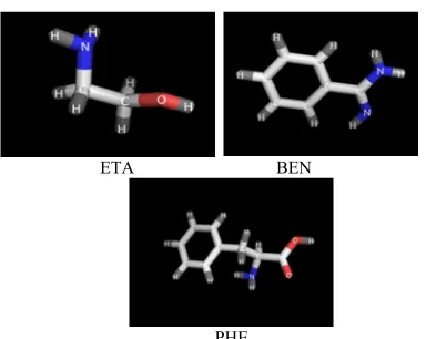
The largest pocket on the surface of thermolysin identified by CASTp server as pocket 48 was chosen as the binding site in this experiment as shown in Figure 1. The molecular structures for the test ligands are shown in Figure 2.
Figure 1: Visualization of thermolysin structure with pocket 48 colored in red.
ETA BEN
[image:3.612.378.460.214.282.2]PHE
Figure 2: Molecular structure of Ethanolamine (ETA), Benzamidine (BEN) and Phenylalanine(PHE)
3.1 Q-learning Agent For Protein-Ligand Docking
The environment for the proposed reinforcement learning agent to work on is the protein and ligand’s three-dimensional positions, rotation and torsions angles. The agent can be viewed as a ‘navigator’ exploring the space of these variables and learning to adjust the values to find optimal ones.
3.1.1 State representation
[image:3.612.91.289.289.387.2]The state of the agent is the ligand’s root position in three dimensional space, its rotational angle and torsion angles. These variables represent a ligand’s pose at any particular time during optimization. The position variable (x,y,z) is discretized by partitioning the space into grids or cubes of equal length with granularity 0.2Å such as in Figure 3.
Figure 3: Illustration of a ligand's root atom in the center of a box representing the search space. The search space is discretized in every axis directions, four in each x, y and z-axis. This results in 64 possible discretized positions.
The orientation angle of the ligand, the rotation vector [r1,r2,r3]T is discretized into bins of equal
size. The rotation axis is fixed while the rotation angle is let to change in 5° step size. The torsion angle is also represented in similar way. Therefore, the set of all possible state, S is the combination of all the discretized position, orientation and torsion angles: S = P x O x T , where P is the set of all discretized ligand’s root position, O is all discretized ligand’s orientation and T is all the discretized torsion angles.
3.1.2 Action representation
The actions the agent can take are:
1. Moving the position of the root atom: the
three-dimensional space is partitioned into octants as in (). The agent will translate the initial position of the root atom to another position in any of these of octants within 0.2 Å. The new position is calculated by the spherical coordinate formula:
∗ sin cos
∗ sin sin
∗
[image:3.612.90.282.419.572.2]5688
2. Rotating the orientation angle. This is done by
incrementing or decrementing rotation angle by 5°.
3. Rotating the torsion angle. For each torsion
angle, the agent increment and decrement it in similar way with the rotational angle.
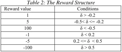
3.1.3 Reward function
The reward function is based on the energy value calculated by Vina scoring function. As better conformation gives lower energy value, therefore positive difference between initial and current conformation entails higher reward value as shown
[image:4.612.94.295.272.358.2]in Error! Reference source not found. below.
Table 2: The Reward Structure
Reward value Conditions
1 δ > -0.2
5 -0.5< δ <= -0.2
100 δ < -0.5
-1 δ < 0.2
-5 0.2 <= δ < 0.5
-100 δ > 0.5
3.1.4 Q-learning with Torsion Prototypes
Even with the state and action space discretized as described, the size of the state-action space is still very large and limits the application of Q-learning. To limit the number of state-action space, we apply Kanerva coding technique described by [15] in this work. With Kanerva coding, a subset of S is selected. However, in QLTP, only a subset of the discretized torsion angle was chosen and this subset will be adapted based on visit frequency. This subset taken from the discretized torsion angle is called torsion prototypes. To generate a torsion prototype, a bin is randomly picked from each discretized torsion angle. Subsequent torsion prototypes will be generated the same way while making sure there will be no duplicates. The torsion prototypes will then replace the discretized torsion angles in the state representation. For example, say a ligand has three torsion angles and discretized each torsion angles to three bins as illustrated in Table 3. Four torsion prototypes could be generated such as in Table 4. Torsion prototype 1 is generated by taking the first bin from the first and the second torsion angle and taking the second bin from the third torsion angle.
Table 3: An Example of Prototyping a Ligand's Torsion Angles with Three Equal-Distance Bins
Bin 1 Bin 2 Bin 3
Discretized torsion 1
0.1 – 0.18 0.18 – 0.26 0.26 – 0.34
Discretized
torsion 2 0.03 – 0.11 0.11 – 0.18 0.18 – 0.26
Discretized torsion 3
0.05 – 0.13 0.13 – 0.21 0.21 – 0.29
Table 4: An Example of Four Unique Torsion Prototypes Based on Discretization shown in Table 3.
Prototype 1 Prototype 2 Prototype 3 Prototype 4
0.1 – 0.18 0.18 – 0.26 0.1 – 0.18 0.26 – 0.34
0.03 – 0.11 0.11 – 0.18 0.11 – 0.18 0.18 – 0.26
0.13 – 0.21 0.05 – 0.13 0.21 – 0.29 0.21 – 0.29
The number of visits for each prototype is kept and is incremented for the prototype activated for an update. Now every time a state transition occurs, the value of the Q-table, , is updated by the function:
Q(s,a) = Q(s,a) + (s,a)[ (r + . , ) - Q(s,a))]
where , is the membership function assigning the pair (s,a) to the prototypes. For any state s and torsion prototype p, , is 1 if p is adjacent to the (s,a)’s contained torsion prototype, and let , = 0 if otherwise. Two state-action pair is adjacent to each other if the torsion prototype contained in them are different only in 1 place. For example, a torsion prototype p1=<a,b,c>
would be adjacent to torsion prototypes <a,b,d>, <a,d,c> and <d,b,c> but not to something like <a,d,e>. So everytime an update occurs, the algorithm will update multiple (s,a) in look up table and the number of visits for each of them is incremented. A maximum number of visits to any (s,a) is observed. Prototypes that are visited too frequently will be splitted and those prototypes visited infrequently will be deleted. Frequently visited prototypes are split into one or more new prototype by randomly choosing a bin from the original torsion prototype and increment or decrement its value. Doing so will generate new prototypes adjacent to the original and thus make the frequently visited region more refined with prototypes able to distinguish between different state-action pairs. The probability of deleting a prototype is based on the exponential function,
5689
4. EXPERIMENTS AND RESULTS
4.1 Experiment I
In order to test the proposed agent effectiveness, AutoDock Vina program was run first and the resulting conformations were set as the goal conformations for each ligand. The agent will have to explore the conformational space and learn to find these goals. The effectiveness of QLTP was tested with different values for its parameters: discount factor, learning rate and granularity-cubes-number of prototypes value combination (gcp), by observing the rate of its reward accumulation over time in docking three ligands: ethanolamine, benzamidine and phenylalanine to thermolysin. QLTP agent will start its search from two random initial conformations generated in the vicinity of each of the goal conformations. QLTP was run ten times to get the average cumulative reward over number of episodes.
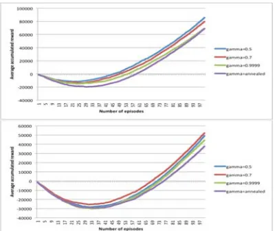
4.1.1 Effect of discount factor
[image:5.612.313.517.101.273.2]Figure 4, 5 and 6 show the average cumulative reward for docking ETA, BEN and PHE respectively. QLTP managed to recoup its cost of learning in every instance. The difference of performance when using the different values of discount factor tested is not remarkable. In docking smaller ligands such as ETA and BEN, QLTP learns to find better conformation giving bigger rewards faster as evidence in the sharp upward curves of the graphs. In docking PHE from the first starting conformation, QLTP was slow in finding the better conformations although managed to find some later in the episodes.
[image:5.612.313.513.311.481.2]Figure 4: Effect of Discount Factor in Docking ETA from Two Starting Conformations
Figure 5: Effect of Discount Factor in Docking BEN from Two Starting Conformations.
Figure 6: Effect of Discount Factor in Docking PHE from Two Starting Conformations
4.1.2 Effect of learning rate
[image:5.612.90.290.535.703.2]5690
[image:6.612.316.517.265.564.2]Figure 7: Effect of Learning Rate in Docking ETA from Two Starting Conformations
Figure 8: Effect of Learning Rate in Docking BEN from Two Starting Conformations
Figure 9: Effect of Learning Rate in Docking PHE from Two Starting Conformations
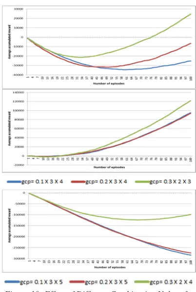
4.1.3 Effect of granularity-cube-number of torsion prototypes (GCP)
The results in Figure 10 show that different
combination of granularity, discretization and number of prototypes give significantly different performance. As learning progress, QLTP accumulates higher rewards and regain its cost of exploration. In docking ETA, QLTP accumulates higher rewards when using g=0.3, c=2, p=3. This means a coarser granularity value, small number of discretized position variable and small number of torsion prototypes enables the agent to improve its policy. This is true for both BEN and PHE as well.
Figure 10: Effect of Different Combination Values for Granulation Size, Discretization Size and Number of
Torsion Prototype
4.2 Experiment II
[image:6.612.88.292.293.462.2] [image:6.612.88.292.500.667.2]5691 summarized in Table 5 below. “Diff” is the average
of the difference between the lowest energy found by QLTP by the end of its search from each of the ten starting conformation and the goal’s conformation energy. The number in the bracket is the standard deviation. In docking ETA, the value for Diff found are positive in every case indicating the inability of QLTP to find matching or better conformation then goal’s conformation found by Vina. However, with 5000 steps, QLTP found one close enough to the goal. In contrary, QLTP managed to find better conformation with energy lower than the goal’s conformation energy for both BEN and PHE in every number of steps tested.
Table 5: Comparison of QLTP Effectiveness in Three Ligands with 500, 1000 and 5000 Time Steps. The goal
energy found by Vina was -2.554, -5.098 and -6.085 kcal/mol for ETA, BEN and PHE respectively.
#Steps Ligand Lowest Diff
500 ETA -2.521 0.107(0.09)
BEN -5.492 -0.28(0.08)
PHE -6.210 -0.047(0.06)
1000 ETA -2.519 0.088(0.06)
BEN -5.513 -0.307(0.06)
PHE -6.227 -0.061(0.06)
5000 ETA -2.531 0.049(0.04)
BEN -5.522 -0.339(0.05)
PHE -6.229 -0.073(0.06)
The reliability of QLTP is measured in its ability in consistently finding similar low energy conformations by running ten QLTP runs for one starting conformation and calculating its average. This is repeated to every starting conformation and recording the overall mean for every case of number of steps tested and the standard deviations. The standard error of the overall mean then recorded by dividing the overall mean’s standard deviations to the square root of the number of starting conformations used. Table 6 summarizes the
reliability of QLTP. Generally, with larger time steps, the overall mean and the standard error decrease in docking every ligand. This proves with larger number of steps, QLTP improves the quality of the conformation it finds. This also proves it finds conformations with similar energy consistently every run. In the case of ETA, given even the largest time steps, a 95% confidence interval for the mean of energy found by QLTP would be in between -2.48 to -2.41 kcal/mol. Therefore, QLTP most probably would not match the goal’s conformation energy which is -2.554kcal/mol. In docking BEN, QLTP would
always find conformation better than the goal’s conformation, even when using number of steps as low as 500. In docking PHE, the mean of the energy QLTP would find in 5000 steps is between -6.15 to -6.07 kcal/mol at 95% confidence. This indicates, armed with 5000 number of steps, most of the time QLTP would find conformation with energy better or similar than the goal’s conformation energy. This is not the case for 500 and 1000 number of steps.
Table 6: The average energy found by QLTP from ten different starting conformations averaged over ten runs
with 500, 1000 and 5000 number of steps.
#Steps Ligand Mean Std. Error
500 ETA -2.342 0.06
BEN -5.299 0.033
PHE -6.055 0.027
1000 ETA -2.394 0.029
BEN -5.355 0.024
PHE -6.074 0.023
5000 ETA -2.45 0.0173
BEN -5.402 0.021
PHE -6.11 0.019
5. CONCLUSIONS
5692 such as the magnitude of the translation and angle of rotation for a more efficient exploration. Implementation of other reinforcement learning methods could be done and compared using the proposed representation. As the starting conformations in the experiments were generated by Vina, therefore a fast global optimization algorithm such as genetic algorithm is needed to provide these starting points for the QLTP agent. Further work can be done in combining QLTP with these global optimization techniques.
ACKNOWLEDGEMENT
This work has been supported by Fundamental Research Grant Scheme (FRGS) by the Malaysia Ministry of Higher Education.
REFERENCES:
[1] C. Watkins and P. Dayan, “Q-learning,” Machine Learning, vol. 8, no.3-4, 1992, pp. 279-292.
[2] F.J. Solis and R.J.B. Wets, “Minimization by random search techniques,” Mathematics of Operations Research, vol. 6, no.1, 1981, pp. 19-30.
[3] H.M. Chen, B.F. Liu, H.L. Huang, S.F. Hwang and S.Y. Ho, “SODOCK: Swarm Optimization for Highly Flexible Protein-Ligand Docking,” Journal of Computational Chemistry, vol. 28, no.2, 2007, pp. 612-623. [4] G.M. Morris, D.S. Goodsell, R.S. Halliday, R.
Huey, W.E. Hart, R.K. Belew and A.J. Olson, “Automated Docking Using a Lamarckian Genetic Algorithm and an Empirical Binding Free Energy Function,” Journal of Computational Chemistry, vol. 19, no.14, 1998, pp. 1639-1662.
[5] M.C. Ng, S. Fong and S.W. Siu, “PSOVina: The hybrid particle swarm optimization
algorithm for protein–ligand
docking,” Journal of Bioinformatics and Computational Biology, vol. 13, no. 3, 2015, p. 1541007.
[6] E. Atilgan and J. Hu, “Efficient Protein-Ligand Docking Using Sustainable Evolutionary Algorithms,” 10th International Conference on Hybrid Intelligent Systems, 2010, pp. 113–118.
[7] O. Trott and A.J. Olson, “Autodock Vina: Improving the Speed and Accuracy of Docking with a New Scoring Function, Efficient Optimization, and Multithreading,” Journal of Computational Chemistry, vol. 31, no.2, 2010, pp. 455-461.
[8] D.W. Miller and K.A. Dill, “Ligand binding to proteins: The binding landscape model,” Protein Science, vol. 6, no.10, 1997, pp. 2166-2179.
[9] A. Tovchigrechko and I.A. Vakser, “How Common is the Funnel-Like Energy Landscape in Protein-Protein Interactions?,” Protein Science, vol. 10, no.8, 2001, pp. 1572-1583.
[10] R. D. Smith, A. L. Engdahl, J. B. Dunbar and H. A. Carlson, “Biophysical Limits of Protein-Ligand Binding,” Journal of Chemical Information and Modeling,” vol. 52, no. 8, 2012, pp. 2098–2106.
[11] Y.N. Dauphin, R. Pascanu, C. Gulcehre, K. Cho, S. Ganguli and Y. Bengio, “Identifying and attacking the saddle point problem in high-dimensional non-convex optimization,” Advances in Neural Information Processing Systems, 2014, pp. 2933-2941.
[12] J. Tavares, S. Mesmoudi and E.G. Talbi, “On the Efficiency of Local Search Methods for the Molecular Docking Problem,” European Conference on Evolutionary Computation, Machine Learning and Data Mining in Bioinformatics, Springer Berlin Heidelberg, 2009, pp. 104-115.
[13] M.B.A. Rahman, A.H. Jaafar, M. Basri, R.N.Z.R.A Rahman, A.B. Salleh and H.A. Wahab, “Design of Novel Semisynethetic Metalloenzyme from Thermolysin,” BMC Systems Biology, vol. 1, no.1, 2007.
[14] H.M. Berman, J. Westbrook, Z. Feng, G. Gilliland, T.N. Bhat, H. Weissig, I.N. Shindyalov and P.E. Bourne, “The Protein Data Bank,” Nucleic Acids Research, vol. 28, no.1, 2000, pp. 235-242.
[15] M. Allen and P. Fritzsche, “Reinforcement Learning with Adaptive Kanerva Coding for Xpilot Game AI,” IEEE Congress of Evolutionary Computation (CEC), 2011, pp. 1521-1528.