CORRELATES OF SUCCESS IN JAVA PROGRAMMING: PREDICTING THE PERFORMANCE OF STUDENTS IN A JAVA COURSE FROM THE RESULTS OF LOWER LEVEL COURSES

1856

MODELING THE STRUCTURE OF SOCIAL NETWORKS BY

USING THE PYTHAGOREAN SPIRAL

1_{IZEM ACIA,} 2_{WAKRIM MOHAMED,} 3_{GHADI ABDERRAHIM}

1,2_{Dept. of Mathematics & Informatics (LabSI), FSA- Ibn Zohr University, Morocco}

3_{Dept. of Computer Science(LIST), FST- Abdelmalek Essaadi University, Morocco}

E-mail: 1_{[email protected],} 2_{[email protected],} 3_{[email protected]}

ABSTRACT

Since the good representation of the complex networks structure can effectively communicate more information and can help explore them and understand their behaviors, the purpose of this paper is to present and model the structure of social networks.

Mathematical concepts can be a powerful tool for modeling. However, complex networks in the real world are far too complicated to model in their entirety. Therefore, it is important to identify the information that the generated model may help illustrate.

In the present work, we use the spiral of Pythagoras and a combination of mathematical concepts in pre-topology, graph theory and fuzzy logic to generate two different models: the Rings Model and the Member-ship Matrix. The first proposed model has a geometric representation which makes all the nodes visible and every direct link between two nodes illustrates the number of, direct and indirect, paths that connect them and the cost of each one. The second proposed model is a matrix where every column depicts the relation between the corresponding node and the rest of the network.

The most important benefit of the models presented in this paper is that they allow the human eye to get information about the strength of connection between the nodes, of complex networks, in an easy and fast way.

Keywords: Spiral of Pythagoras, Pretopology, Fuzzy Logic, Social Networks, Complex Networks,

Mathematical Modeling, Matrix, Rings Model.)

1. INTRODUCTION

With the huge size of complex networks, it is necessary to represent their structure with models that have a high readability. A model with a high readability is a model that optimizes the search for information.

In the last decades, many complex networks lend themselves to the use of graphs [1-6] for analyzing and modeling their structure. Usually, the vertices of the graph stand for the nodes of the network and the edges between vertices stand for (possible) interactions between the nodes.

We cite for example [7-17]: Erdos-Renyi random graph model, Barabasi-Albert model, Watts-Strogatz Small World model, The Kleinberg model. However, all these models have some limitations. In other words, in the Erdos-Renyi model the edges are randomly added, the selected edge had the probability p to be selected and the next edge has also the probability p to be selected. This makes p a constant not a probability.

Moreover, the both implementations (the model A and the model B) of Albert and Barabasi model (BA) fail to represent real-world networks because:  The model A retains growth but does not

include preferential attachment. The probability of a new node connecting to any pre-existing node is equal.

 The model B retains preferential attachment but eliminates growth. The model begins with a fixed number of disconnected nodes and adds links, preferentially choosing high degree nodes as link destinations.

However, the growth and the preferential attachment are simultaneously needed in real networks. Therefore, neither the number of nodes nor the probability can be fixed.

Additionally, in the Small World model, of Watts-Strogatz, the number of nodes and the probability, to rewire edges, are fixed. Therefore, this model does not represent the growth and the dynamics that characterize the real-world networks.

1857

Figure 2: The Construction of the Pythagorean Spiral.

In other word, the more the number of nodes and the number of edges increase the more complicated the structure of the model becomes.

A part of the modeling process is determining the answer we are searching and the type of structure or operation we are looking for. Therefore, the main objective of this paper is to propose mathematical models that represent the structure of social networks and optimize the search of information. In the present work, we illustrate two mathematical models with high readability: The Rings Model and the Membership Matrix.

The first proposed model has a geometric representation which makes all the nodes visible. In addition, just by looking at the edge that connects the nodes X and Y we may know how many paths connect them and the cost of each one.

The second proposed model has a matrix representation where every column depicts the relation between the corresponding node and the rest of the network.

The remainder of this paper is structured as follows. Section 2 reviews the mathematical concepts used in the proposed models. Section 3 provides a historical overview about our assumption of using the Pythagorean spiral. Section 4 and 5 present the proposed models. Section 6 illustrates an application of the Rings model in the real-world networks.

2. DEFINITIONS

2.1 The K-th Order Neighbor

Let the nodes B, C, D, E, F, G and H be the neighbors of the node A (See Figure 1). According

to the degree of neighborhood, the neighbors of A can be classified into: The 1st _{order neighbors (B, C}

and D), the 2nd _{order neighbors (E, F and G) and the}

3th _{order neighbors (H).}

Figure 1: The K-th Order Neighbor.

2.2 The Membership Function

The membership function for a fuzzy set A on the universe of discourse X is defined as

µA: X → [0,1], where each element of X is mapped to a value between 0 and 1. This value, called the membership degree, quantifies the grade of membership of the element in X to the fuzzy set A [18-20].

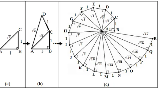
2.3 The Construction of the Pythagorean Spiral

Figure 2 depicts the drawing process of the Pythagorean spiral [21-23].

3. HISTORICAL OVERVIEW

The main reasons for using the Pythagorean spiral in the present work can be summarized in defining a distance equal to one for neighbors nodes that are directly connected and greater or

1st _{order neighbors}

2nd _{order neighbors}

1858

Figure 3: The Pythagorean Spiral

equal to one between a node and its K-th order neighbor.

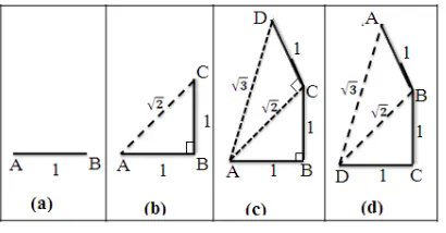
In other words, suppose we have 4 vertices: A, B, C and D where B is a neighbor of A, C is a neighbor of B and D is a neighbor of C. Unlike an ordinary graph where the nodes are drawn anywhere and the lengths of edges have no importance, in this paper we took into account the graph spatialization (how the nodes occupy the space) by using the Pythagorean spiral. For example, in order to draw the graph corresponding to the 4 vertices above we do the following steps:

 B is a neighbor of A: To draw B, we draw a line segment onto A (See Figure 3-(a)).  C is a neighbor of B: To draw C, we add

another line segment onto B with a right angle (See Figure 3-(b)).

 D is a neighbor of C: To draw D, we add

another line segment onto C, the end of the hypotenuse AC, with a right angle (See Figure 3-(c)).

By looking at Figure 3-(c), A and B (Resp. B and C (Resp. D and C)) are direct neighbors, thus:

𝑑 𝐴, 𝐵 𝑑 𝐵, 𝐶 𝑑 𝐶, 𝐷 1

A and C (Resp. A and D) are not direct neighbors: C (Resp. D) is the 2nd _{(Resp. 3}th_{) order neighbor of}

A, thus:

d A, C √2 and d A, D √3

Likewise if we search the distance between D and its neighbors we need to take D as a root (instead of A) as shown in figure 3-(d). Hence we have:

𝑑 𝐷, 𝐶 1, 𝑑 𝐷, 𝐵 √2, 𝑑 𝐷, 𝐴 √3

Last but not least, our assumption of using the Pythagorean spiral in modeling, complex networks and particularly social networks, faced two

problems: The first is that a node (individual, page, event), in general, has many neighbors as in the case of social networks. The second is the cycles. We get to handle these problems as follows. Concerning the first issue, we look at the Pythagorean spiral in three dimensions instead of two dimensions. In other words:

 For the 1st _{order neighbors of the root node of}

the spiral: The only condition between this special node and its 1st _{order neighbors the}

distance must be 1. By going back to the previous example and looking at Figure 3-(a), it is clear that B can be any point of the set of points that consists the sphere with A center and 1 radius. Hence, the root node A can have an infinite number of (direct) neighbors.  For the remaining nodes of the spiral: By

looking at Figure 3-(b), to draw C the first order neighbor of B we needed to fulfill two conditions:

𝑑 𝐵, 𝐶 1 and 𝐵𝐶 ⊥ 𝐴𝐵 .

Thus C can be any point of the set of points that consists the perimeter of the base (directrix ) of the right circular cone with apex A and height AB and radius BC=1 as shown in Figure 4-(a). Hence, B can have an infinite number of (direct) neighbors. Likewise to draw D the first order neighbor of C (Figure 3-(c)) we needed to fulfill two conditions:

𝑑 𝐶, 𝐷 1 and 𝐷𝐶 ⊥ 𝐴𝐶

Thus, D can be any point of the set of points that consists the directrix (perimeter of the base) of the right circular cone with apex A and height AC and radius CD=1( see Figure 4-(b)). Hence, C can have an infinite number of (direct) neighbors. In brief, the number of neighbors is not a problem, we can draw as much as we need of neighbors.

Concerning the second issue (the cycles): We assume that an individual A will be represented by a set of nodes {A1, A2, A3,….,An} (where n is an

integer greater than or equal to 1) rather than one node.

1859

Figure 4: Infinite Number Of Neighbors

Figure 5:The New Form Of The Spiral

4. THE FIRST PROPOSED MODEL: THE

RINGS MODEL

4.1 Model Description

Our first model relies on the assumption that a social network can be represented by isolated components. In each component, every pair of nodes (A,B) is connected by at least one edge, the cost of each edge that connect the pair (A,B) is d(A,B) where d(A,B) is the distance between A and B that is gotten by using the Pythagorean spiral. Furthermore, each component takes the shape of a ring.

4.2 New Form of the Pythagorean Spiral

The direct use of the Pythagorean spiral in the distances calculation process gave us irreadble structure. Thus, we make the following simplification:

 We straighten the spiral (see Figure 5-(a)).  We replace edges with arrows to indicate the

direction of the Pythagorean spiral construction.

 We add columns: the first column contains the root node of spiral, the kth_{column contains the}

(k-1)th _{order neighbors of the root node.}

 By looking at Figure 4, we deduct that the distance between the root node of the Pythagorean spiral (for example the node A in Figure 3) and its kth _{order neighbors is √k 1.} Thus, in the top of the kth _{column we put}

√k 1 (see Figure 5-(b)).

In the remainder of this paper, we use the new form of the Pythagorean spiral (see Figure 5-(b)) instead of the real form.

4.3 The Exploring Rule

In the exploring process, we use the following rule:

Let A and B be nodes. A and B belong to the same spiral S: If A is already displayed as a direct or an indirect predecessor of B, A must not be added as a successor of B in S.

4.4 The Distances Calculation Algorithm

Figure 6 depicts the algorithm that we use to calculate the distances between a node and its k-order neighbor.

4.5 Illustration: Calculation Of The Distances

1860 Initial conditions

Figure 6: The Distances Calculation Process

Table 1: Relations between individuals

Individual Friends

A

H J M

H A _N

J A _F

F _M J

M A _F

N H

4.5.1 Calculation of the distances between F and

his neighbors.

To calculate the distance between the individual F and his neighbors, we have to make the node F the root node of the Pythagorean spirals, thus we put it in the first column (See Figure 7-(a)). The individual F has 2 friends (See Table 1): J and

M, we put them in the second column (See Figure 7-(a)) and we assign to them the index 1: As we already assume that an individual X will be represented by a set of nodes {X1, X2,…,Xn}, thus

for every new occurrence of X we assign a new value to the X index.

Next, we explore the first order neighbors of each node in the second column (Breadth-first search):

 For J1, J has 2 friends: F and A, they are the 1st order neighbors of the node H1 and the 2nd order neighbors of the node A. Therefore, in the 3th _{column we write A}

1 but according to the

Exploring Rule we cannot write F: F is

already the predecessor of J1 (See Figure 7-(b)). We use 1 as index for A1 because this is the first occurrence of A.

 For M1, M has 2 friends: A and F thus we add

A2 to the graph seen in Figure 7-(a), but according to the Exploring Rule we do not add F: F is already a predecessor of M1 (See Figure 7-(a)). Hence we get the graph presented in Figure 7-(b). We use 2 as index for A2 because this is the second occurrence of

A.

Next, we explore the nodes of the third column and we deploy their first order neighbors. For the node A1 (Resp. A2), A has 3 friends: J, H and M. By applying the Exploring Rule, we add just M2 and H1 (Resp. J2 and H2) to the graph seen in Figure 7-(b) because J (Resp. M) is already a direct predecessor of A1 (Resp. A2) in the spiral F→

J1→A1 (Resp. F→M1→A2). Thus we get the graph presented in Figure 8.

Next, we explore the nodes of the 4th _column

and deploy their first order neighbors: Selection of a node X

Exploring the neighborhood of X

Concatenation of the distances

End

Figure 7 : Calculation Of Distances Between F And His Neighbors

1861  For M2, M has 2 friends: A and F. By looking

at the spiral or the path F⟶J1⟶A1⟶M2, M2 has already A (Resp. F) as direct (Resp. indirect) predecessor. Thus according to the Exploring Rule, we add nothing to the graph seen in Figure 8.

 For H1 (Resp. H2), H has 2 friends: A and N. Thus according to the Exploring Rule, weadd just N1 (Resp. N2) as shown in Figure 8.

 For J2, like M2, J has two friends but they are already predecessors of the node J2. Thus according to the Exploring Rule, we add nothing to the graph seen in Figure 8.

Next, we explore the nodes of the 5th _column

and deploy their first order neighbors. For N1 (Resp.

N2), the individual N has only H as a friend. But according to the Exploring Rule, we add nothing to the graph seen in Figure 8 because N1 (Resp. N2) has already H as a predecessor (see Figure 8).

Finally, according to the exploring rule we cannot add more nodes to the graph presented in Figure 9. Therefore we get to the end of the exploring process.

By looking at Figure 9, the graph is composed of 4 Pythagorean spirals (in the new form):

 The first spiral: F →J1→A1→M2.

 The second spiral: F →J1→A1→H1→N1.

 The third spiral: F →M1→A2→ H2→N2.

 The fourth spiral: F →M1→A2→J2.

Furthermore, in the graph presented in Figure 9, M

has 2 occurrences: M1 and M2, that means anything shared by F can reach M in 2 different ways: The first path is F→M1, the length of this path is

d(F,M1)=1. The second path is F →J1→A1→M2, the length of this path is d(F,M2)=√2.

Moreover, these paths are independent: if F deletes

M from his contact list, M can still receive what F

shared because the fact that F deletes M from his contact list is actually deleting the first path. Thus if

F really want to delete any exchange or sharing with M, he needs to delete all the gateways that connect him to M in other words he has to delete J

from his contact list.

Last but not least, the graph seen in Figure 9 helps us determinate the distance between F and his neighbors (See Table 2). For example, the distances between F and the nodes of the 4th _{column (see}

Figure 9) are:

d(F,M2)=d(F,H1)=d(F,H2)=d(F,J2)=√3.

H has 2 occurrences in this column thus we write the both distances d(F,H1) and d(F,H2) in the table of distances (Table 2) because the paths

F→J1→A1→H1 and F→M1→A2→H2 are independent.

Table 2: Distances between F and his neighbors

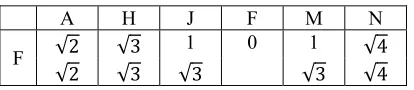
A H J F M N

F √2 √3 1 0 1 √4

√2 √3 √3 √3 √4

4.5.2 The results of distances calculation

We follow the same process used in the calculation of distance between F and his neighbors to calculate the distances between A (Resp. H

(Resp. J (Resp. M (Resp. N)))) and his neighbors. Then we concatenate the tables of distances. In the end, we get the distances presented in Table 3.

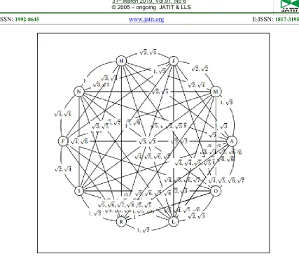
4.6 Rings Model

On the one hand, by looking at Table 3 we notice that the distance between every pair of nodes is finite. Thus, we represent the connection between every pair of individuals as shown in Figure 10.

Figure 10: Connection Between Two Nodes, The

Distance Between A And J Has 2 Values: 1 And √3,

These Values Are Used As The Cost Of The Edge (A,J)

1862

Figure 11: The Rings Models Table 3: Distances Between Every Pair Of

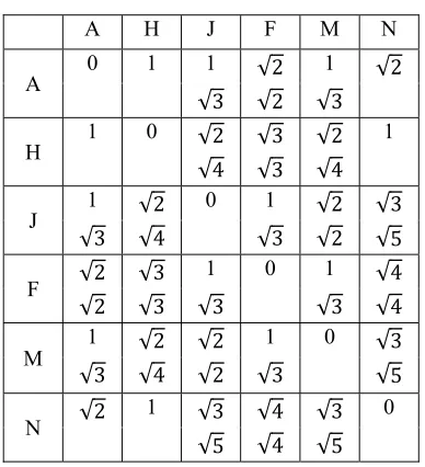
Individuals

A H J F M N

A 0 1 1 √2 1 √2

√3 √2 √3

H 1 0 √2 √3 √2 1

√4 √3 √4

J 1 √2 0 1 √2 √3

√3 √4 √3 √2 √5

F √2 √3 1 0 1 √4

√2 √3 √3 √3 √4

M 1 √2 √2 1 0 √3

√3 √4 √2 √3 √5

N √2 1 √3 √4 √3 0

√5 √4 √5

In addition, by arranging the nodes as a ring and adding all the possible connections we get a ring where every pair of nodes is connected as shown in Figure 11-a.

In the other hand, we assume that the structure of social networks is composed of isolated rings: For illustration purposes, we consider the neighborhood relations presented in Table 4. Then

we calculate the distance between the individuals of this table (See Table 5) and we create the corresponding rings model (See Figure 11-b).

In the end, we can see that there is no neighborhood relation between the individuals of Table 1 and the individuals of Table 4. No neighborhood relation no edge between the both rings. Hence, we get two isolated rings (See Figure 11).

Table 4: Neighborhood Relations

Individual Friends

I R _L

R

L O I

L _R I

O R

Table 5: Distance between neighbors

I R L O

I 0 1, √2 1, √2 √2,√3

R 1, √2 0 1, √2 1

L 1, √2 1, √2 0 _√2, √3

1863

Figure 12: Evolution of the network structure: After merging, the two rings become one big ring

Moreover, if the individual I and the individual J become friends, the two rings seen in Figure 11 are merged. Therefore we get a big ring as shown in Figure 12.

4.7 Discussion

The main goal of modelling is to amplify cognition by reducing the search for information and encoding them. The rings model is not a perfect model but it is better than the existed structure models because it makes the structure of social network more readable and it provides interesting information. In other words:

 The geometric presentation of the model makes the nodes and the edges visible despite the size of the network, we can follow every edge from source to destination.

 The global structure of social network is composed of isolated rings. The size of the rings may change by individuals (or nodes)

joining in or withdrawing from one or more rings.

 Parallel calculation is done in the generation process. In other words, the calculation of the distances between :

 The individual F and his neighbors.  The individual A (Resp. H (Resp. J (Resp.

M (Resp. N )))) and his neighbors.

can be done in parallel.

 In the update process, the previous structure is

used.

 The cost of the edge (A, B) may show how closely and strongly connected A and B are.  The diameter of the ring R is:

(max({d(X,Y) /X, Y ∈ R}))2

1864

 KX = n-1 where n is the number of the ring nodes.

 If X and Y belong to the same ring R then

KX = KY.

It (the passive degree) shows how large the node network is. In other words, if the active degree tells us how many first order neighbors the node has, the passive degree tells us how many Kth _order neighbors it has.

5. THE SECOND PROPOSED MODEL: THE

MEMBERSHIP MATRIX

5.1 Definition Of The Membership Function

We define the membership function F as follows:

 FX(X) = 1

 FX(Y) = 0 if X and Y are isolated (there is no direct or indirect neighborhood relation between X and Y).

 FX(Y)= _, if Y is the K-th order neighbor of X.

Where FX(Y) is the membership degree of Y to the neighborhood of X.

5.2 Constructing The Membership Matrix

5.2.1 Algorithm

Figure 13 depicts the algorithm that we use to generate the Membership matrix.

5.2.2 Illustration

To construct the Membership matrix, we follow the following steps:

1) From Table 3 (Resp. Table 5), we extract the table of minimum distances (see Table 6 (Resp. Table 7)) by keeping just the minimum value of each cell.

2) We calculate the degree of membership of an individual to the neighborhood of another individual. For example, to calculate the degree of membership of the individuals of Table 1 and Table 4 to the neighborhood of the individual A, we use the following relations (Definition of our membership function F) :

 FA (A) =1.

 FA(Y) =0 if A and Y are isolated.

 FA(Y )= _, If Y is a K-th order neighbor of A.

Figure 13: The Generation Process Of The Membership Matrix

Table 6: The Minimum Distances

A H J F M N

A 0 1 1 _√2 1 _√2

H 1 0 _{√2 √3 √2} 1

J 1 _√2 0 1 _{√2 √3}

F _{√2 √3} 1 0 1 _√4

M 1 _{√2 √2} 1 0 _√3

N _√2 1 _{√3 √4 √3} 0

Table 7: The Minimum Distances

I R L O

I 0 1 1 _√2

R 1 0 1 1

L 1 1 0 _√2

O _√2 1 _√2 0

Thus:

 FA(A) = 1,

FA(M) = FA(J) = FA(H) = _, =1

 FA(F) = FA(N)= _, = _, =_√

 There is no neighborhood relation between A

and the individuals of Table 4. So A and I

(Resp. R (Resp. L (Resp. O))) are isolated. Thus: FA(I) = FA(L) = FA(O) = FA(R) = 0.

We organize these values into a table (See Table 8). Initial conditions

Generation of the minimum distances

Calculation of the membership degrees

Concatenation of the membership degrees

1865

Table 9 : Membership Matrix

A H J F M N I R L O

A 1 1 1 1

√2

1 1

√2

0 0 0 0

H 1 1 1

√2 1 √3

1 √2

1 0 0 0 0

J 1 1

√2

1 1 1

√2 1 √3

0 0 0 0

F 1

√2 1 √3

1 1 1 1

√4

0 0 0 0

M 1 1

√2 1 √2

1 1 1

√3

0 0 0 0

N 1

√2

1 1

√3 1 √4

1 √3

1 0 0 0 0

I 0 0 0 0 0 0 1 1 1 1

√2

R 0 0 0 0 0 0 1 1 1 1

L 0 0 0 0 0 0 1 1 1 1

√2

O 0 0 0 0 0 0 1

√2

1 1

√2

1 Table 8: The Membership Degrees To

The Neighborhood Of A

A A FA (A) =1 H FA (H) =1

J 1

F 1

√2

M FA (M)=1

N 1

√2

I 0

R 0

L 0

O 0

Likewise, we calculate the membership degree to the neighborhood of every individual. In the end we get the matrix presented in Table 9.

5.3 Discussion

Unlike the Adjacency Matrix, the Membership Matrix provides more information about the relation between a node and the rest of the network. For example, By just using the Membership Matrix presented in Table 9 and by looking at the first column of this matrix (the column corresponding to A) we can deduct:

 H is a direct neighbor of A because FA(H)=1.

 N is an indirect neighbor of A because 0 < FA(N) < 1.

 The individual J is near to A than N because

FA(J) > FA(N) (1 > _√ ).

 The individual I is not connected to the network of A because FA(I) = 0.

 Every individual X who has 0 FA(X) 1 can receive what the individual A shares.

 Every individual X who has FA(X) = 0 can never receive what the individual A shares.

6. APPLICATION

1866

Figure 14: The rings model of Morocco's national airline routes: The airport ESU and OZG are isolated: they are not connected to the national airports of Morocco however they are connected to the international airports. This graph is obtained by using JUNG JAVA graph library [27].

complicated to model in their entirety. Hence, when generating models, it is necessary to determine what information we are seeking to get just by looking at the model.

The airline routes network is one of the most complex networks used nowadays. Drawing directly this network gives a complicated structure (review the graph [24]). This structure may become more complicated if the direction of the routes was taken into account and every possible route between two airports was represented.

The proposed models are not limited to social networks, they can be used to represent the structure of many other complex networks. Therefore, as the first application of the rings model in the real-world networks, we generate the rings model of Morocco's (Resp. Tunisia's) national airline network.

An airline network is composed of directional airline routes which connect two locations. Thus, from routes.dat [25-26], we extract the graph

𝐺 𝑉, 𝐸 (Resp. 𝐺′ 𝑉′, 𝐸′ ) where:

 V (Resp. V′) is the set of airports codes inside Morocco (Resp. Tunisia).

 𝐸 (Resp. 𝐸′) is the set of arrows (X, Y) where X

is the source airport code and Y is the destination airport code.

Then we use 𝐺 𝑉, 𝐸 (Resp. 𝐺′ 𝑉′, 𝐸′ ) to generate the rings model presented in Figure 14 (Resp. Figure 15) and we opt to display the square of the distances to avoid the approximation of the square root.

In addition, to illustrate the evolution of the network, we add the direct routes between the two countries. Therefore, the rings presented in Figure 14 and Figure 15 are merged as shown in Figure 16.

1867

Figure 16: Evolution of airline network structure of Morocco and Tunisia. This graph is obtained by using JUNG JAVA graph library [27].

Figure 15: The Rings model of Tunisia's national airline routes. This graph is obtained by using JUNG JAVA graph library [27].

connection between national airports of Morocco is faster by using the rings model (Figure 14) than using the graph presented in Figure 17. Despite the fact that the both graphs (Figure 14 and Figure 17) are using the same database (Routes.dat [25]). For instance: By dragging and zooming out the nodes GLN and VIL, we may know how many paths can be used to go from the airport GLN to the airport VIL (Resp. from VLN to GLN) and the cost of each path without looking at the rest of the graph. For example, in Figure 14, the cost of the arrow (GLN,VIL) is 3;4;5 that means to go from the airport GLN to the airport VIL, by using the national airline network of Morocco, there are 3 different paths: the first (Resp. the second (Resp. the third)) path uses 2 (Resp. 3 (Resp. 4)) intermediary airports.

1868

Figure 17: National airline routes network of Morocco. This graph is extracted from [26].

Therefore, the human eye may get information about the connection between two nodes in an easy and fast way as already illustrated in Figure 14.

7. CONCLUSION

Complex network modeling has a rich history. In this paper, we have presented two new models: The Rings model and the Membership Matrix, the both represent the structure of complex networks in particularly social networks.

The most important characteristic of these models (The Rings model and the Membership Matrix) is the high readability. In other words, the huge size of complex networks makes the human eye struggle to get information about the connection between nodes. However, the mathematical models proposed in the present work focus on highlighting the information that the human eye may look for which helps making its (the human eye) searching easier and faster.

ACKNOWLEDGMENT

Financial support provided by CNRST, funded by Moroccan government, is gratefully acknowledged. The authors also wish to thank an anonymous reviewer for his helpful comments on an earlier draft of the manuscript.

REFERENCES:

[1] Karin R Saoub, A tour through graph theory, CRC Press 2018, Chapter 1, pp 1-34.

[2] Reinhard Diestel, Graph theory, Springer-Verlag Berlin Heidelberg 2017, Chapter 1, pp 1-33.

[3] Koushik Sinha, Graph theory basic terminology part I, Lecture notes, Southern Illinois University, 2017.

[4] Saidur Rahman, Basic graph theory, Springer 2017, Chapter 1-3, pp 9-37.

[5] Narsingh Deo, Graph theory with applications to engineering and computer science, Dover Publications 2016, Chapter 1-2, pp 14-35

.

1869 [7] Newman, M. E. J, The structure and function

of complex network,. SIAM Review, Jun 2003, 45(2), pp 167-256.

[8] Emmanuelle LEBHAR, Routing algorithms and random models for small world graphs, Thesis, 2005, ENS of Lyon France, Chapter 0-1, pp 5-24.

[9] Jorg Reichardt, Structure and function of complex modular Networks, Thesis, university of Bremen, Germany. August 2006. [10] Remco van der Hofstad, Random graphs and complex networks, 2016, Course notes

available at

http://www.win.tue.nl/\~rhofstad/NotesRGCN .html

[11] Maarten van Steen, An introduction to graph theory and complex networks, Lexington, January 2010.

[12] PA. Noel, Stochastic dynamics on complex networks. Thesis, LAVAL University QUEBEC 2012, Chapter 1, pp 1-20. Chapter 6-7, pp 79-120.

[13] Vincent LEVORATO, Modeling complex networks: Pretopology and Application, Thesis, University of Paris 8, 2008. Chapter 1, pp 22-37.

[14] Ernesto Estrada, The structure of complex networks theory and applications, Oxford University Press, 2011, Chapter 12, pp 233-256.

[15] ACC Coolen, Theory of complex networks, Module 6CCMCS02/7CCMCS02, Lecture Notes, department of mathematics King's College London, 2015, pp 48-69.

[16] Guido Caldarelli, Alessandro Vespignani, Large scale structure and dynamics of complex networks from information technology to finance and natural, Complex Systems and Interdisciplinary Science Vol. 2, , 2007, pp 17-34.

[17] Vito Latora, Vincenzo Nicosia, Giovanni Russo, Complex networks: Principles, methods and applications, Cambridge University press 2017. Chapter 3-6, pp 69-256.

[18] Bryan Klingenberg,Paulo.F. Ribeiro. Fuzzy Logic, Calvin College Engineering Department.

Review:https://www.calvin.edu/~pribeiro/othrlnks/ Fuzzy/fuzzysets.htm

[19] Sunil Mathew, John N. Mordeson, Davender S. Malik, Fuzzy graph theory, Springer 2018, Chapter 1, pp 11-12.

[20] D.S. Hooda, Vivek Raich, Fuzzy logic models and fuzzy control: An introduction, Alpha Science 2017, Chapter 1-2, pp 1-54.

[21] Sparks J.C, The Pythagorean theorem, Crown jewel of mathematics 2008, Chapter 4, pp 157-165.

[22] Eli Maor, The Pythagorean theorem A 4,000-year history, Princeton University Press 2007, Chapter 9, pp 126-127.

[23] Glenda Lappan, James T. Fey, William M. Fitzgerald , Susan N. Friel, Elizabeth Philips, Looking for Pythagoras, the Pythagorean theorem, Prentice Hall, Connected Mathematics (2) 2005, Chapter 4, pp 46-48.

[24]Airline Routes Network, review:

https://openflights.org/demo/openflights-routedb-2048.png

[25] Routes.dat (2014) is available in: https://openflights.org/

[26] Airline Route Mapper (2014), review: https://arm.64hosts.com/