www.hydrol-earth-syst-sci.net/21/345/2017/ doi:10.5194/hess-21-345-2017
© Author(s) 2017. CC Attribution 3.0 License.
Formulating and testing a method for perturbing precipitation time
series to reflect anticipated climatic changes
Hjalte Jomo Danielsen Sørup1,2, Stylianos Georgiadis1,3, Ida Bülow Gregersen4, and Karsten Arnbjerg-Nielsen1,2
1Technical University of Denmark, Global Decision Support Initiative, Lyngby, Denmark 2Technical University of Denmark, Department of Environmental Engineering, Lyngby, Denmark
3Technical University of Denmark, Department of Applied Mathematics and Computer Science, Lyngby, Denmark 4Ramboll Danmark A/S, Department of Climate Adaptation and Green Infrastructure, Copenhagen, Denmark
Correspondence to:Hjalte Jomo Danielsen Sørup ([email protected])
Received: 25 September 2016 – Published in Hydrol. Earth Syst. Sci. Discuss.: 6 October 2016 Revised: 3 January 2017 – Accepted: 4 January 2017 – Published: 20 January 2017
Abstract.Urban water infrastructure has very long planning horizons, and planning is thus very dependent on reliable es-timates of the impacts of climate change. Many urban water systems are designed using time series with a high tempo-ral resolution. To assess the impact of climate change on these systems, similarly high-resolution precipitation time series for future climate are necessary. Climate models can-not at their current resolutions provide these time series at the relevant scales. Known methods for stochastic downscaling of climate change to urban hydrological scales have known shortcomings in constructing realistic climate-changed pre-cipitation time series at the sub-hourly scale. In the present study we present a deterministic methodology to perturb his-torical precipitation time series at the minute scale to re-flect non-linear expectations to climate change. The method-ology shows good skill in meeting the expectations to cli-mate change in extremes at the event scale when evaluated at different timescales from the minute to the daily scale. The methodology also shows good skill with respect to represent-ing expected changes of seasonal precipitation. The method-ology is very robust against the actual magnitude of the ex-pected changes as well as the direction of the changes (in-crease or de(in-crease), even for situations where the extremes are increasing for seasons that in general should have a de-creasing trend in precipitation. The methodology can pro-vide planners with valuable time series representing future climate that can be used as input to urban hydrological mod-els and give better estimates of climate change impacts on these systems.
1 Introduction
Climate change impacts water management worldwide as the water cycle is an essential part of the climate system. The planning horizon for water infrastructure is often very long, making reliable predictions of future climate crucial (Arnbjerg-Nielsen et al., 2015b). In the design of water in-frastructure, precipitation data are needed. Especially for ur-ban infrastructure the time resolution of precipitation data needed for design and planning is much finer than what is provided by climate models (Berndtsson and Niemczynow-icz, 1988; Schilling, 1991). Hence a lot of effort is put into giving reliable estimates of what the expected change in pre-cipitation will be at these fine scales (Fowler et al., 2007; Kendon et al., 2014; Mayer et al., 2015). Expected changes in precipitation, however, do not translate directly into changes in floods or overflows from structures. To determine these changes, urban hydrological models have to be run, driven by the changed precipitation (Olsson et al., 2009; Willems et al., 2012). By definition, fine-resolution precipitation time series for future climates are not observable, and hence a multitude of statistical approaches have been developed to enable gen-eration of time series with properties that for a large range of metrics have the same characteristics as the expected future precipitation (Willems, 1999; Olsson and Burlando, 2002; Cowpertwait, 2006; Molnar and Burlando, 2008; Burton et al., 2010; Willems et al., 2012; Sørup et al., 2016a).
changes in seasonal or yearly precipitation (Boberg et al., 2010). This is a problem often solved by weather generators or other similar downscaling techniques (Fowler et al., 2007; Burton et al., 2010), but these often have difficulty in present-ing realistic time series at the sub-hourly to hourly timescales relevant for urban infrastructure (Segond et al., 2006; Ver-hoest et al., 2010; Sørup et al., 2016a). Several studies have tested the applicability of Markov models for simulation of high-resolution precipitation series (Srikanthan and McMa-hon, 1983; Thyregod et al., 1998; Ailliot et al., 2009; Gelati et al., 2010; Sørup et al., 2012). The approach has the ad-vantage that realistic chronology is created in the output. However, for very high resolutions the sensing method of the gauge may have an impact on the signal, giving an upper bound to the temporal resolution of the model, as has been shown for e.g. tipping bucket gauges (Thyregod et al., 1998; Sørup et al., 2012).
In the present study, we develop and demonstrate a novel non-linear methodology that perturbs existing precipitation time series to reflect complex expectations to precipitation in a changed future climate. The method incorporates regional historical knowledge about precipitation through the use of Intensity-Frequency-Duration (IDF) relationships (WMO, 2009) and knowledge about the expected changes in these due to climate change. Thus, the method generates time se-ries for a changed climate which are chronologically identi-cal to the observations used as input, but perturbed to reflect climate change. These series can be used as input for hy-draulic or hydrologic models where the climate change effect has to be assessed for all possible rain conditions.
The presented methodology is based on the assumption that precipitation can be scaled according to identified expec-tations to climate changes. In its simplest form, this assump-tion is identified as the Delta Change (DC) method (Fowler et al., 2007). The basic assumption is that relative changes in output from climate models might represent expectations to climate change well even though the output itself could be wrongly scaled in absolute values. A more elaborate use of this assumption is provided by Distribution Based Scal-ing (DBS) presented by Yang et al. (2010). In this approach parameters are derived from regional climate model data to estimate present and future distribution functions for rainfall intensities. The relative change in the distribution parameters is applied to a similar distribution function based on obser-vational data. Thereby, perturbation of rainfall intensities due to climate change relies on the rarity of the individual events and changes markedly from average to extreme events with a high impact on hydrological responses of simulation mod-els (van Roosmalen et al., 2011). Unlike the study by Yang et al. (2010), the expected changes in this study are not cal-culated directly using the DC method on Regional Climate Model output; they are derived from comprehensive state-of-the-art studies where all available data are used to determine realistic expectations to changes to precipitation due to
cli-mate change (e.g. Giorgi, 2006; Kendon et al., 2008; Chris-tensen et al., 2015).
2 Methodology
In urban water management, the relevant time frame to con-sider is most often that of the rain event (Willems, 1999). The determination of robust IDF relationships for present climate at the relevant timescales is a prerequisite. For de-veloped countries where high-resolution precipitation is gen-erally available, these two prerequisites are very often met (Arnbjerg-Nielsen et al., 2015a), making the methodology generally relevant. The general flow of the methodology is presented in Fig. 1, and how to proceed with each step is presented in the following sections (2.1–2.5).
2.1 Modelling framework
Let us consider a systemS that describes precipitation over a time period. The original data are expressed as a time se-ries of precipitation intensity over fixed time steps. This time series alternates between a dry period (no precipitation) and a rainy one. A given event is characterised as dry, extreme or non-extreme with respect to the amount of precipitation during the event.
We denote byEthe state space of the systemS, with at least three states, i.e.|E| ≥3. Also letD0,D1andD2be the
non-empty sets of states of dry periods, non-extreme and ex-treme events, respectively, with|D0| =1,|D1| =d1≥1 and
|D2| =d2≥1, i.e. there exists exactly one state for dry
peri-ods,D0=Ddry, but a different number of extreme and
non-extreme states (d1 andd2, respectively) can be defined for
both the non-extreme and extreme events. An extreme event can be further categorised according to the severity of the phenomenon, expressed in terms of the return period of the measured intensity. Non-extreme events can be categorised according to the season in which they appear. Hence, the state spaceEis partitioned into three disjoint subsets as follows:
E=D0∪D1∪D2, (1)
where Di∩Dj =∅, i6=j, ij∈ {0,1,2}. We link the
non-extreme events to the seasonality of the phenomenon and
thusD1=Dwinter, Dspring, Dsummer, Dautumn , that isd1=
4.D2can likewise be partitioned into one or several states
appropriate for describing extreme precipitation which may have different return periods or different hydro-climatic ori-gins. In this study, we use a partition based on return periods withD2=D2, D10, D100 , referring to states that classify
the extremes as either 2-, 10- or 100-year events based on return level.
Add Presentation Title
in Footer via ”Insert”; ”Header & Footer” Define
relevant system
states
Define events and define which states
they individually
belong to
Determine change factors for
system states
Perturb original time
series with change factors given
each event' s state affiliation
Evaluate perturbed time series
against expected
[image:3.612.98.499.66.139.2]change
Figure 1.Flow diagram showing the general process involved in the presented methodology.
– J :=(Jn)n∈N is a Markov chain with state space E,
whereJnis the state of the system at thenth event;
– U:=(Un)n∈N is the sequence of jump times between states with state spaceNandU0=0; and
– Z:=(Zk)k∈N is a discrete-time process with states on
E, withZkto be the state of the system at a time stepk.
The processesJ andZare related through the formula
Zk=JN(k), k∈N, (2)
whereN (k)is the discrete-time counting process of events in [1, k]⊂N, i.e.
N (k):=max{n∈N:Un≤k}. (3)
The corresponding transition matrix of the chain J is very simple. Figure 2b illustrates the evolution of the stochastic system described above.
2.2 Framework for determining state of individual events
There is no unique way to assign a state to an extreme event. In the literature some studies apply hydro-climatic regimes for this classification (Gelati et al., 2010; Svoboda et al., 2016), while others apply event statistics (Madsen et al., 2009; Sørup et al., 2016a). For any given application, the most appropriate classification depends on the data available. In this paper, various methods based on the maximum mean intensities are used to define the event state. For all investi-gated methods the changes to extremes are evaluated by cal-culation of IDF curves based on return levels, zis, at event
level for a selection of return periods,I (WMO, 2009). The return period (T) of individual events across all intensities is determined using the median plotting position (Rosbjerg, 1988):
Tmedian=
Ttotal+0.4
rank−0.3, (4)
whereTtotal is the length of the time series and rank is the
rank number of the individual event.
Using data with observations every minute and a mini-mum dry weather separation between events of 60 min, the mean maximum intensities over 5, 10, 30, 60, 180, 360 and
Intensity
Non−extreme summer event
Non−extreme winter event
2−year extreme event
100−year extreme event Original events
Perturbed events (a)
Time
S
ta
te
sp
a
c
e
, E
(b)
D
dry
D
winter
D
spring
D
summer
D
D
2
D
10
D
100
U0U1 U2 U3 U4 U5 U6 U7 U8 U9
CFsummer
CFwinter
CF2
CF100
autumn
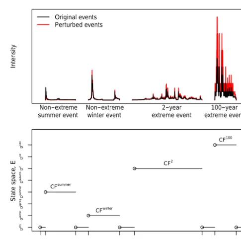
Figure 2. (a)Illustration of the magnitude of perturbation of events for non-extreme summer and winter events as well as 2- and 100-year extreme events, with summer events being perturbed with a factor below 1 and factors for the winter and the extremes being above 1. Factors for extremes are higher than for the winter events, and factors for the very extreme are higher than for the more mod-erate extreme.(b)Illustration of the states associated with the dif-ferent events if they were to happen in the shown chronology; the dry state,Ddry, is present between all wet states.
[image:3.612.307.550.180.422.2]Figure 3.The IDF curve for an extreme event in comparison to the regional IDF curves for 0.5-, 2-, 10- and 100-year return periods, respectively (based on Madsen et al. (2017)).
2.3 Perturbation and change factor
With each event of a time series classified according to a state, the time series can be perturbed using the following methodology linking the time series to the states of the indi-vidual events.
LetRk,k∈N, be the precipitation intensity at time step
k and R:=(Rk)k∈N the corresponding process describing these intensities. The process of perturbed precipitation in each time stepkis denoted byR∗:= Rk∗
k∈N.
Similarly to the state spaceE, we introduce the state space of the change factors, denoted byECF,|ECF| = |E|. We can
then write
ECF=C0∪C1∪C2, (5)
with|C0| =1,|C1| =d1and|C2| =d2.
We consider the process CF:=(CFn)n∈Nwith state space
ECF, where CFn is the change factor at the nth event. Let
W :=(Wk)k∈Nbe the chain, with state spaceECF, of change
factors in time stepsk∈N, that is
Wk=CFN (k) (6)
withN (k)to be the counting process defined in (Eq. 3). Un-der the above notation, the original and perturbed sequences of precipitation,RkandRk∗, are written as
Rk∗=WkRk. (7)
This means that, for a sequence of events, some events will be perturbed more than others, and for extreme cases some might be reduced while others are increased, depending on the local expectations to climate change. Figure 2a shows an example where a non-extreme summer event is perturbed to a lesser volume than the original while a winter non-extreme is increased marginally and both 2- and 100-year extremes are increased considerably more (both in absolute numbers as well as in relative percentages). Figure 2b shows how the state space changes if these four events were to happen chronologically in time with the state jump times marked on thex axis.
2.4 Volume correction based on seasonal dependence of extremes
The extreme part of precipitation is only expected to consti-tute a smaller fraction of the total precipitation volume on an annual basis (Sørup et al., 2016b), but as extreme pre-cipitation is often associated with a particular season (see e.g. Sørup et al., 2012), the volumetric part of the extremes might be higher for sub-annual considerations. This implies that situations where the expectations for changes to the ex-tremes are very different from the expectations to changes to seasonal precipitation have to be handled through volumetric corrections in order to accommodate the fact that both expec-tations to changes in extremes and overall seasonal changes are correct. How to do this best will be very much depen-dent on the local conditions. In our case this is described in Sect. 3.4.
2.5 Evaluation of perturbed time series
The evaluation of the perturbed time series is done against the original time series and against the expected changes.
The average percent-wise difference between the per-turbed return levels, z∗i,j,m, of the modelled time series, Rk∗, perturbed with the time-dependent change factors,Wk,
against the same return levels,zi,j,m, of the original time
se-ries,Rk, multiplied by the target change factor, CFje, can be
defined as
8i,j,m= 1−
z∗i,j,m
zi,j,mCFje
!
100 %, (8)
across all IDF points,i, all extremity levels and seasonality, j, and all perturbed time series,m. A combined skill score, 8, across all considered metrics that describe the average de-viance from the expectations, can then be defined as
8=X
i∈I
X
j∈J
X
m∈M
1−8i,j,m
|I| |J| |M|, (9)
with|I| |J| |M|being the product of the total number of IDF points,I, the total number of extreme levels considered plus seasonality,J, and the total number of time series perturbed, M, as a normalization factor.
2.6 Sensitivity analysis
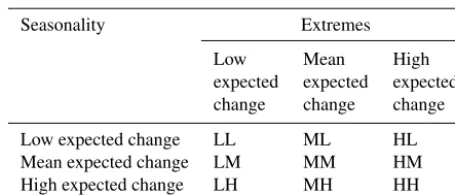
Table 1.Tested combinations of extreme and seasonal changes.
Seasonality Extremes
Low Mean High
expected expected expected change change change
Low expected change LL ML HL
Mean expected change LM MM HM High expected change LH MH HH
3 Case study: Denmark
To showcase the methodology, it is applied to Danish condi-tions where the situation is that complex non-linear changes are expected with respect to precipitation in a changed cli-mate.
3.1 Data
3.1.1 Observational data
Precipitation data from the Danish SVK rain gauge network are used in this study (Mikkelsen et al., 1998; Madsen et al., 2002). For this study 10 time series from different parts of Denmark with lengths of approximately 33 years between 1979 and 2012 are used. To distinguish individual events, a dry weather period between individual events of at least 60 min is applied.
3.1.2 IDF curves
For present climate IDF curves are extracted from a re-gional model for extremes originally developed by Madsen et al. (1998) and updated by Madsen et al. (2009) and Mad-sen et al. (2017). The IDF curves vary across Denmark, but a single mean regional curve is chosen for this study inde-pendently of the location of the gauge considered. Table 2 summarises the IDF values used.
3.1.3 Expectations to climate change
The official recommendations regarding climate change for urban infrastructure in Denmark was determined by Gregersen et al. (2014) on the basis of the ENSEMBLES data set (van der Linden and Mitchell, 2009), with the addition of a few simulations using high-end scenarios. The data set in-dicates that in general precipitation amounts and intensities will increase and that extremes will increase more than the expected mean increases for Denmark. Furthermore, the re-sults show that it is very likely that increases will be more pronounced for the very rare extremes compared to the more frequent extremes. Table 3 sums up these official expecta-tions for the three return periods that has to be assessed in Danish urban hydrological contexts.
In addition, the Danish Meteorological Institute has pub-lished expectations regarding climate change on a seasonal basis (Olesen et al., 2014). The analysis is performed for a range of climate variables and focuses on utilizing the data available in the best possible way to create realistic un-certainty intervals for the expected changes. The estimated change factors for precipitation are based on analysis of the RCP2.6 and RCP8.5 scenarios (Moss et al., 2010), hence a low-end emission scenario and a high-end emission scenario, respectively. Table 4 lists these expectations as well as a sim-ple mean average of the two to represent the mean expected change. To match the change factors for extreme precipita-tion in Gregersen et al. (2014), which primarily is based on the more average emission A1B scenario (Nakicenovic et al., 2000), simple scaling of the seasonal expectations to a mid-point is applied, as scalability has been shown to be a valid assumption across most scales and most indices (Christensen et al., 2015). The A1B scenario does not lie exactly in the middle between the RCP2.6 and RCP8.5 scenarios, but def-initely somewhere between these, and the original estimates from Olesen et al. (2014) are kept as low and high expected changes for the sensitivity analysis.
3.2 Defining states
For Denmark the state space (Eq. 1) is defined with a total of eight states based on the expectations to climate change listed in Tables 3 and 4 with four seasonal states defined for the non-extreme events and three states for the different extreme event levels:
E= {Ddry, Dwinter, Dspring, Dsummer, Dautumn, D2, D10, D100}.
(10) Correspondingly the change factors used to perturb the time series are, as a starting point, determined based on the mean expectations listed in Tables 3 and 4.
3.3 Determining state of individual events
For the determination of the state of the individual ex-treme events four different selection criteria are investi-gated, with the purpose of defining a representative re-turn period for each event. All points mentioned refer to the return periods of the events intensity points, T = {T5, T10, T30, T60, T180, T360, T720}, shown in a situation as
depicted in Fig. 3:
Criterion A The maximum return period is used to define the return period of the whole event (based on one point);
Tevent=T1∗=maxT. (11)
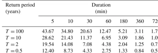
Table 2.IDF intensities (µm s−1) for various return periods for Denmark extracted from the model presented by Madsen et al. (2017).
Return period Duration
(years) (min)
5 10 30 60 180 360 720
T =100 43.67 34.80 20.63 12.47 5.21 3.11 1.72
T =10 28.62 21.43 11.37 6.95 3.09 1.86 1.09
T =2 19.54 14.08 7.08 4.38 2.04 1.25 0.75
[image:6.612.162.436.90.182.2]T =0.5 12.40 8.73 4.33 2.75 1.33 0.84 0.51
Table 3.Expected changes in extreme precipitation for Denmark. All values from Table 1 of Gregersen et al. (2014).
Change factor 2-year 10-year 100-year
for extreme event event event
precipitation (–) (CF2) (CF10) (CF100)
Low expected change 1.0 1.0 1.0 Mean expected change 1.2 1.3 1.4 High expected change 1.45 1.7 2.0
Tevent=
1 3
X3 i=1T
∗
i , (12)
whereT2∗ andT3∗are the second and third maxima, respec-tively, i.e.T2∗=max{T\T1∗}andT3∗=max{T\(T1∗∩T2∗)}. Criterion C The mean of all the return periods is used to
define the events (based on all seven points):
Tevent=T. (13)
Criterion D A customised step-wise threshold selection cri-terion is constructed where the event-specific IDF curve is compared to regional IDF levels.
Criterion D is important to test as this allows for construc-tion of a criterion that is closely linked to specific knowl-edge on the place-specific precipitation dynamics, i.e. for how many duration points on the IDF curve a given return period has to be exceeded for it to be essential for the classi-fication of the event.
Following these selection criteria, four different systems, Si, i∈ {A, B, C, D}, are constructed and analysed.
OptionsSAtoSCare straightforward based on Eqs. (11)–
(13), but option SD is determined specifically for the case
study. Table 5 summarises the methodology for option SD
used in this study; specifically it is reflected that for very extreme events, fewer durations have to be extreme for the event as a whole to be considered extreme compared to the more moderate 2-year return level.
3.4 Volume correction based on seasonal dependence of extremes
In previous studies using the SVK data set, it has been shown that
1. the extreme events account for at most 25 % of the to-tal rainwater volume on an annual basis (Sørup et al., 2016b), and
2. the extreme events occur mostly in the summer season (Sørup et al., 2012).
Furthermore, in the summer season the expected seasonal change (−10 %) differs mostly from the expected change in extremes (+20–40 %); see Tables 4 and 3, respectively. Based on this information the seasonal change factor for non-extreme summer events has to be adjusted to reach the overall change factors reported in Table 4. We esti-mate a partition between non-extreme and extreme events of
{fnon-extreme, fextreme} = {0.8,0.2}, and the change factor for
2-year events, CF2, is used to represent the extremes as the largest seasonal volume by far is for the more frequent ex-tremes (Sørup et al., 2016b). In this way the change factor for summer, CFsummer, can be adjusted from its value listed in Table 4 (0.9) as
CFsummeradjusted=CF
summer−CF2f extreme
fnon-extreme
=0.9−1.2·0.2
0.8 =0825. (14) In other words the change factors for non-extreme summer events are modified from−10 to−17.5 % in order to com-pensate for the positive change of+20–40 % to the extremes occurring in the summer period. For the other seasons such an adjustment is not needed.
4 Results
4.1 Evaluation of selection criteria
The 10 time series are perturbed using the four different state selection criteria (SA−SD) and the evaluation metric is
Table 4. Expected seasonal changes to precipitation in Denmark based on data from Table 5 of Olesen et al. (2014) and linearly scaled midpoint values.
Change factor for seasonal Winter Spring Summer Autumn precipitation (–) (CFwinter) (CFspring) (CFsummer) (CFautumn)
Low expected change (RCP2.6) 1.0 1.0 1.0 1.0
Mean expected change 1.1 1.05 0.9 1.05
[image:7.612.96.501.201.301.2]High expected change (RCP8.5) 1.2 1.1 0.8 1.1
Table 5.Selection criterionSDfor choosingTevents at event level.
ATeventis chosen of a If Or
2-year event At least four points from the event have At least two points from the event have a return period above 0.5 years a return period above 2 years
10-year event At least three points from the event have At least two points from the event have a return period above 2 years a return period above 10 years 100-year event At least three points from the event have At least two points from the event have
a return period above 10 years a return period above 100 years non-extreme event None of the above criteria are met
Table 6.Calculated skill scores,8, for the four selection criteria A– D calculated using Eq. (10).
SA SB SC SD
8 9.3 % 8.5 % 12 % 6.4 %
selection criterionSDoutperforms the other alternatives even
though all selection criteria seem reasonable, as all estimated deviances are below 13 % of the expected changes.
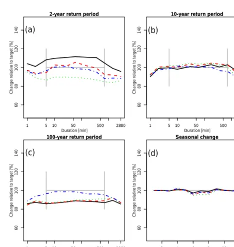
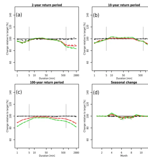
In order to study the performance for each state, we con-struct the skill score variable of Eq. (8) and plot it against the duration for the individual extremes and against months for seasonal precipitation (Fig. 4). Plotted this way 100 % represents a perfect fit, 0 % represents no change and ev-erything positive represents a change in the right direction. For the 2-year return levels both state selection criteria SB
and SD perform similarly and with a relative change close
to 100 %. State selection criterion SA overestimates the
2-year return level by approximately 10 % on average and state selection criterion SCunderestimates it with a similar
mag-nitude, which still corresponds to a positive change for the events (Fig. 4a). For the 10-year return level, all state se-lection criteria perform similarly very well (Fig. 4b). When the 100-year return level is evaluated, the reason for crite-rionSD’s better overall performance becomes clear: it is the
only criterion that does not systematically underestimate this return level (Fig. 4c). Even so, all criteria produce results where the direction of change is correct. Given the inherent uncertainty in estimating the actual levels of such events, ob-taining close to 85 % of the expected change is considered good. With respect to the seasonal behaviour, all state
selec-1 5 10 50 500
60
80
100
120
140
2-year return period
Duration [min]
Change relativ
e to target [%]
(a)
2880 1 5 10 50 500
60
80
100
120
140
10-year return period
Duration [min]
Change relativ
e to target [%]
(b)
2880
1 5 10 50 500
60
80
100
120
140
100-year return period
Duration [min]
Change relativ
e to target [%]
(c)
2880 2 4 6 8 10 12
60
80
100
120
140
Seasonal change
Month
Change relativ
e to target [%]
(d)
SA SB SC SD
Figure 4.Performance of the different selection criteria,SA−SD, in
producing(a)2-year extremes,(b)10-year extremes,(c)100-year extremes and(d) seasonal changes according to the perturbation schemes listed in Tables 3 and 4.
tion criteria have approximately the same performance at a level close to 100 % (Fig. 4d).
[image:7.612.308.549.325.579.2] [image:7.612.95.240.358.389.2]Table 7.Calculated skill scores,8, for selection criterionSDfor the
nine different sensitivity scenarios listed in Table 1 calculated using Eq. (9).
8 Extremes
Low Mean High
Seasonality Low 0.0 % 6.0 % 8.6 % Mean 1.0 % 6.4 % 8.8 % High 1.2 % 6.3 % 8.8 %
(5–720 min). At the minute scale, this is of minor importance, but at 2 days (2880 min) the tendency is very robust across different state selection criteria and extremity levels. This is most likely because these average extreme events are caused by several events with dry periods in between. Hence the in-dividual events are each assessed to be non-extreme and they are adjusted towards lower volumes, even though combined they are rather extreme.
4.2 Sensitivity analysis with selection criterion D The sensitivity analysis is carried out for the best state se-lection criterion only, i.e. criterion SD. The resulting skill
scores for the nine individual sensitivity scenarios are listed in Table 7. The highest sensitivity is found when changing between the different extreme precipitation scenarios, with a large increase in the metric when moving from low to mean scenarios and also a notable increase when moving from mean to high scenarios. As such the performance of the methodology drops with the magnitude of the expected changes to extremes, but even for the high extremes the per-formance is similar to the perper-formance of state selection cri-teria SA toSD in Table 6. The methodology, on the other
hand, shows very little sensitivity to the variation in expec-tations to seasonal changes, not even for the combination where the difference between expectations to seasonal sum-mer precipitation (−20 %) and the extremes become very high.
For all extreme (+45–100 %) indices (Fig. 5a–c), the sen-sitivity of the expected change in extremes is notable and, especially for the 100-year return level, it is clear that per-formance drops with increased magnitude of the expected changes to extremes (Fig. 5c), but only to levels compara-ble to that of the state selection criteriaSA−SCas shown in
Fig. 4. Again, the performance for 2-day events (2880 min) is worse than average, as also seen in Fig. 4. For seasonality (Fig. 5d), the general picture is that the sensitivities of both expectations to seasonality and extremes are of less impor-tance and at a similar level, which in general is a lower level than the one observed for the three extreme indices.
1 5 10 50 500
60
80
100
120
140
2-year return period
Duration [min]
Change relativ
e to target [%]
(a)
2880 1 5 10 50 500
60
80
100
120
140
10-year return period
Duration [min]
Change relativ
e to target [%]
(b)
2880
1 5 10 50 500
60
80
100
120
140
100-year return period
Duration [min]
Change relativ
e to target [%]
(c)
2880 2 4 6 8 10 12
60
80
100
120
140
Seasonal change
Month
Change relativ
e to target [%]
(d)
[image:8.612.75.259.107.181.2]LL LM LH ML MM MH HL HM HH
Figure 5.Performance of selection criterionSDfor different
param-eter values as specified in Table 1 for(a)2-year extremes,(b) 10-year extremes,(c)100-year extremes and(d)seasonal changes un-der climate change.
5 Discussion
The proposed framework is very flexible and the separation of dry, non-extreme and extreme weather makes it possi-ble to very effectively perturb time series to reflect differ-ent changes in differdiffer-ent categories. The presdiffer-ented case study uses eight states to distinguish between different levels of ex-tremes and different seasons and is able to produce time se-ries that satisfactorily represent the expected changes listed in Tables 3 and 4. For other places a different number of states could be relevant and the seasonal partition could be different depending on the local climate and expectation to climate change. The proposed modelling framework fully supports these spatial variations.
Four different state selection criteria over specified event durations are tested in the present study (see Sect. 2.2), as these covered realistic possibilities for the data set used in this study and the focus on urban hydrology. As such, differ-ent state selection criteria for differdiffer-ent evdiffer-ent durations could be relevant in different contexts and could, as illustrated by state selection criterionSD, be specified as very subjective
and case-specific criteria. In this study, the subjective state selection criterionSDoutperforms the other criteria (see
per-formance, pointing to criterionSBas being a good onset for
investigating data sets where no presumptions exist and no case-specific criterion can be constructed.
All state selection criteria showed a drop in performance for longer duration events than the ones used in the method-ology; this is likely due to the used event definition with a minimum of 60 min of dry weather between individual events, which will mean that very long lasting extremes are likely split into several events and therefore not identified as extremes. A different event definition with a longer minimum dry period between events could probably partly solve this, but it would reduce the number of events markedly and in-crease the chance of small events close to extremes being seen as part of the extreme, with a somewhat false classifica-tion as a consequence.
The methodology is relatively sensitive to the magnitude of the perturbation factors (see Sect. 4.2), but the sensitiv-ity is not very dominant and is only at the same size as the sensitivity of the different state selection criteria. Also, the methodology does not address the possibilities of changes to dry spells or changes to the occurrence rate of extremes in general. A future research direction could be to study how the state selection criteria along with the semi-Markov system applied here can be used to generate fully stochastic time se-ries where both the inter-event time and the occurrence prob-ability of the extreme states will be included as criteria that can be changed to meet the expectations to climate change.
6 Conclusions
The proposed methodology is a promising way of creating artificially perturbed precipitation time series, which can rep-resent a changed climate and be used as input in hydrologic and hydraulic models. The methodology perturbs existing time series based on a semi-Markov system where precipi-tation time series are split into events characterised as dry, extreme or non-extreme. The wet events are divided into dif-ferent states based on an Intensity-Duration-Frequency re-lationship based state selection criterion. Of the four tested state selection criteria, the case-specific ones show the best results, but the more general criteria too could be of use when less knowledge about the precipitation regime is available. The sensitivity of the methodology was tested against very different expectations to climate change, both with respect to seasonal changes and changes to extremes, and is generally very robust, also regarding seasons where the general change is negative while the expectation to extremes is positive. The produced time series satisfactorily reproduce changes across all seasons and across all levels of extremes relevant for ur-ban hydrology.
7 Data availability
The data set used is a product of The Water Pollution Committee of The Society of Danish Engineers made freely available for research purposes. Access to data is governed by the Danish Meteorological Institute, and they should be contacted for enquiries regarding data ac-cess at https://www.dmi.dk/erhverv/anvendelse-af-vejrdata/ spildevandskomiteens-regnmaalersystem/.
Competing interests. The authors declare that they have no conflict
of interest.
Edited by: C. Onof
Reviewed by: two anonymous referees
References
Ailliot, P., Thompson, C., and Thomson, P.: Space-time modelling of precipitation by using a hidden Markov model and censored Gaussian distributions, J. Roy. Stat. Soc. C-App., 58, 405–426, doi:10.1111/j.1467-9876.2008.00654.x, 2009.
Arnbjerg-Nielsen, K., Funder, S. G., and Madsen, H.: Identifying climate analogues for precipitation extremes for Denmark based on RCM simulations from the ENSEMBLES database, Water Sci. Technol., 71, 418–425, doi:10.2166/wst.2015.001, 2015a. Arnbjerg-Nielsen, K., Leonardsen, L., and Madsen, H.:
Evaluat-ing adaptation options for urban floodEvaluat-ing based on new high-end emission scenario regional climate model simulations, Clim. Res., 64, 73–84, doi:10.3354/cr01299, 2015b.
Barbu, V. and Limnios, N.: Semi-Markov Chains and Hidden Semi-Markov Models toward Applications: Their Use in Re-liability and DNA Analysis, Springer, New York, NY, USA, doi:10.1007/978-0-387-73173-5, 2008.
Berndtsson, R. and Niemczynowicz, J.: Spatial and temporal scales in rainfall analysis: Some aspects and future perspectives, J. Hy-drol., 100, 293–313, doi:10.1016/0022-1694(88)90189-8, 1988. Boberg, F., Berg, P., Thejll, P., Gutowski, W. J., and
Chris-tensen, J. H.: Improved confidence in climate change projec-tions of precipitation further evaluated using daily statistics from ENSEMBLES models, Clim. Dynam., 35, 1509–1520, doi:10.1007/s00382-009-0683-8, 2010.
Burton, A., Fowler, H. J., Blenkinsop, S., and Kilsby, C. G.: Down-scaling transient climate change using a Neyman-Scott Rectan-gular Pulses stochastic rainfall model, J. Hydrol., 381, 18–32, doi:10.1016/j.jhydrol.2009.10.031, 2010.
Cowpertwait, P. S. P.: A spatial-temporal point process model of rainfall for the Thames catchment, UK, J. Hydrol., 330, 586–595, doi:10.1016/j.jhydrol.2006.04.043, 2006.
Christensen, O. B., Yang, S., Boberg, F., Maule, C. F., Thejll, P., Olesen, M., Drews, M., Sørup, H. J. D., and Christensen, J. H.:. Scalability of regional climate change in Europe for high-end scenarios, Clim. Res., 64, 25–38, doi:10.3354/cr01286, 2015. Fankhauser, R.: Influence of systematic errors from tipping bucket
rain gauges on recorded rainfall data, Water Sci. Technol., 37, 121–129, doi:10.1016/S0273-1223(98)00324-2, 1998.
downscaling techniques for hydrological modelling, Int. J. Cli-matol., 27, 1547–1578, doi:10.1002/joc.1556, 2007.
Gelati, E., Christensen, O. B., Rasmussen, P. F., and Rosbjerg, D.: Downscaling atmospheric patterns to multi-site precipitation amounts in southern Scandinavia, Hydrol. Res., 41, 193–210, doi:10.2166/nh.2010.114, 2010.
Giorgi, F.: Climate change hot-spots, Geophys. Res. Lett., 33, L08707, doi:10.1029/2006GL025734, 2006.
Gregersen, I. B., Madsen, H., Linde, J. J., and Arnbjerg-Nielsen, K.: Opdaterede klimafaktorer og dimensionsgivende regninten-siteter (Updated climate factors and design rain intensities) – Spildevandskomiteen, Skrift nr. 30, The Danish Water and Wastewater Committee under the Danish Engineering Soci-ety, Copenhagen, Denmark, https://ida.dk/sites/prod.ida.dk/files/ svk_skrift30_0.pdf (last access: 21 December 2016), 2014 (in Danish).
Kendon, E. J., Rowell, D. P., Jones, R. G., and Buonomo, E.: Ro-bustness of future changes in local precipitation extremes, J. Cli-mate, 21, 4280–4297, doi:10.1175/2008JCLI2082.1, 2008. Kendon, E. J., Roberts, N. M., Fowler, H. J., Roberts, M. J., Chan, S.
C., and Senior, C. A.: Heavier summer downpours with climate change revealed by weather forecast resolution model, Nature Climate Change, 4, 570–576, 2014.
Madsen, H., Mikkelsen, P. S., Rosbjerg, D., and Harremoes, P.: Estimation of regional intensity-duration-frequency curves for extreme precipitation, Water Sci. Technol., 37, 29–36, doi:10.1016/s0273-1223(98)00313-8, 1998.
Madsen, H., Mikkelsen, P. S., Rosbjerg, D., and Harremoes, P.: Regional estimation of rainfall intensity-duration-frequency curves using generalized least squares regression of partial du-ration series statistics. Water Resour. Res., 38, 21-1–21-11, doi:10.1029/2001wr001125, 2002.
Madsen, H., Arnbjerg-Nielsen, K., and Mikkelsen, P. S.: Update of regional intensity-duration-frequency curves in Denmark: Ten-dency towards increased storm intensities, Atmos. Res., 92, 343– 349, 2009.
Madsen, H., Gregersen, I. B., Rosbjerg, D., and Arnbjerg-Nielsen, K.: Regional frequency analysis of short duration rainfall ex-tremes in Denmark from 1979 to 2012, Water Sci. Technol., in review, 2017.
Mayer, S., Maule, C. F., Sobolowski, S., Christensen, O. B., Sørup, H. J. D., Sunyer, M., Arnbjerg-Nielsen, K., and Barstad, I.: Identifying added value in high-resolution cli-mate simulations over Scandinavia, Tellus A, 67, 24941, doi:10.3402/tellusa.v67.24941, 2015.
Mikkelsen, P. S., Madsen, H., Arnbjerg-Nielsen, K., Jørgensen, H. K., Rosbjerg, D., and Harremoës, P.: A rationale for using lo-cal and regional point rainfall data for design and analysis of urban storm drainage systems, Water Sci. Technol., 37, 7–14, doi:10.1016/s0273-1223(98)00310-2, 1998.
Molnar, P., and Burlando, P.: Variability in the scale prop-erties of high-resolution precipitation data in the Alpine climate of Switzerland, Water Resour. Res., 44, W10404, doi:10.1029/2007wr006142, 2008.
Moss, R. H., Edmonds, J. A., Hibbard, K. A., Manning, M. R., Rose, S. K., van Vuuren, D. P., Carter, T. R., Emori, S., Kainuma, M., Kram, T., Meehl, G. A., Mitchell, J. F. B., Nakicenovic, N., Ri-ahi, K., Smith, S. J., Stouffer, R. J., Thomson, A. M., Weyant, J. P., and Wilbanks, T. J.: The next generation of scenarios for
climate change research and assessment, Nature, 463, 747–756, doi:10.1038/nature08823, 2010.
Nakicenovic, N., Alcamo, J., Davis, J., de Vries, B., Fenhann, J., Gaffin, S., Gregory, K., Grübler, A., Jung, T. Y., Kram, T., Le-bre La Rovere, E., Michaelis, L., Mori, S., Morita, T., Pepper, W., Pitcher, H., Price, L., Riahi, K., Roehrl, A., Rogner, H.-H., Sankovski, A., Schlesinger, M., Shukla, P., Smith, S., Swart, R., van Rooijen, S., Victor, N., and Dadi, Z.: Special report on emis-sion scenarios. A special report of Working Group III for the Intergovernmental Panel on Climate Change, Cambridge Univer-sity Press, New York, 2000.
Olesen, M., Madsen, K. S., Ludwigsen, C. A., Boberg, F., Chris-tensen, T., Cappelen, J., ChrisChris-tensen, O. B., Andersen, K. K., and Christensen, J. H.: Fremtidige klimaforandringer i Danmark (Future climate changes in Denmark), Danmarks Klimacenter rapport nr. 6 2014, Danish Meteorological Institute, Copen-hagen, Denmark, https://www.dmi.dk/fileadmin/user_upload/ Rapporter/DKC/2014/Klimaforandringer_dmi.pdf (last access: 21 December 2016), 2014 (in Danish).
Olsson, J. and Burlando, P.: Reproduction of temporal scaling by a rectangular pulses rainfall model, Hydrol. Process., 16, 611–630, doi:10.1002/hyp.307, 2002.
Olsson, J., Berggren, K., Olofsson, M., and Viklander, M.: Apply-ing climate model precipitation scenarios for urban hydrological assessment: a case study in Kalmar City, Sweden, Atmos. Res., 92, 364–375, doi:10.1016/j.atmosres.2009.01.015, 2009. Rosbjerg, D.: Defence of the median plotting position, Progress
Re-port – Institute of Hydrodynamics and Hydraulic Engineering, Technical University of Denmark, 1988.
Schilling, W.: Rainfall data for urban hydrology: what do we need?, Atmos. Res., 27, 5–22, doi:10.1016/0169-8095(91)90003-F, 1991.
Segond, M.-L., Onof, C., and Wheater, H. S.: Spatiat-temporal dis-aggregation of daily rainfall from a generalized linear model, J. Hydrol., 331, 674–689, doi:10.1016/j.jhydrol.2006.06.019, 2006.
Sørup, H. J. D., Madsen, H., and Arnbjerg-Nielsen, K.: De-scriptive and predictive evaluation of high resolution Markov chain precipitation models, Environmetrics, 23, 623–635, doi:10.1002/env.2173, 2012.
Sørup, H. J. D., Christensen, O. B., Arnbjerg-Nielsen, K., and Mikkelsen, P. S.: Downscaling future precipitation extremes to urban hydrology scales using a spatio-temporal Neyman-Scott weather generator, Hydrol. Earth Syst. Sci., 20, 1387–1403, doi:10.5194/hess-20-1387-2016, 2016a.
Sørup, H. J. D., Lerer, S. M., Arnbjerg-Nielsen, K., Mikkelsen, P. S., and Rygaard, M.: Efficiency of stormwater control mea-sures under varying rain conditions: Quantifying the Three Points Approach (3PA), Environ. Sci. Policy, 63, 19–26, doi:10.1016/j.envsci.2016.05.010, 2016b.
Srikanthan, R. and McMahon, T. A.: Sequential generation of short time-interval rainfall data, Nord. Hydrol., 14, 277–306, 1983. Sunyer, M. A., Madsen, H., Rosbjerg, D., and Arnbjerg-Nielsen,
Svoboda, V., Hanel, M., Máca, P., and Kyselý, J.: Projected changes of rainfall event characteristics for the Czech Republic, J. Hydrol. Hydromech., 64, 415–425, doi:10.1515/johh-2016-0036, 2016. Thyregod, P., Arnbjerg-Nielsen, K., Madsen, H., and Carstensen,
N. J.: Modelling the embedded rainfall process using tipping bucket data, Water Sci. Technol., 37, 57–64, doi:10.1016/S0273-1223(98)00316-3, 1998.
van der Linden, P. and Mitchell, J. F.: Ensembles: Climate change and its impacts: Summary of research and results from the en-sembles project, Technical Report, Met Office Hadley Centre, Exeter, UK, 2009.
van Roosmalen, L., Sonnenborg, T. O., Jensen, K. H., and Christensen, J. H.: Comparison of Hydrological Simulations of Climate Change Using Perturbation of Observations and Distribution-Based Scaling, Vadose Zone J., 10, 136–150, doi:10.2136/vzj2010.0112, 2011.
Verhoest, N. E. C., Vandenberghe, S., Cabus, P., Onof, C., Meca-Figueras, T., and Jameleddine, S.: Are stochastic point rainfall models able to preserve extreme flood statistics?, Hydrol. Pro-cess., 24, 3439–3445, doi:10.1002/hyp.7867, 2010.
Willems, P.: Stochastic generation of spatial rainfall for ur-ban drainage areas, Water Sci. Technol., 39, 23–30, doi:10.1016/s0273-1223(99)00212-7, 1999.
Willems, P., Arnbjerg-Nielsen, K., Olsson, J., and Nguyen, V.-T.-V.: Climate change impact assessment on urban rainfall extremes and urban drainage: methods and shortcomings, Atmos. Res., 103, 106–118, doi:10.1016/j.atmosres.2011.04.003, 2012. WMO: Guide to hydrological practices. Volume II: Management
of Water Recourses and Application of hydrological practices, WMO report 168, 6th edn., World Meteorological Organization, Geneva, Switzerland, p. 302, 2009.